
Cover: original generated illustration. Several instruments observe the same uncertain path. It is a metaphor, not market data.
RSI falls below 30. Price slips beneath the lower Bollinger Band. Another red candle closes.
It is tempting to read the screen as an invitation: the market has fallen too far, so a rebound must be close. Then price makes another low. The oscillator remains extreme. The supposedly stronger signal produces another losing entry.
The arithmetic may be working exactly as intended. The problem is the conclusion attached to it.
A technical indicator measures something about observations already available. Turning that measurement into a forecast, and then into a trade, requires additional claims. Each claim needs its own evidence.
This article grew out of a comparative study of 81 named tools and variations, a review of 16 research papers, and a limited set of reproducible calculations. The question was practical: what is the smallest set of tools that helps us interpret a difficult market without manufacturing confidence?
The answer is provisional. Price structure and a volatility scale provide useful descriptions. Data quality, event awareness and execution constraints determine whether those descriptions can support a decision. No combination in this project earned endorsement as a reliably profitable 15-minute WTI or MCX system.
That qualification matters. The available data supported daily spot-price information tests and a small, named-contract CL intraday calculation demonstration. They did not support a multiyear intraday futures backtest after realistic costs.
The five steps hidden inside a trading signal
Consider the sentence, “RSI is oversold, so I should buy.” It compresses five different things:
| Step | What it might say | What still needs establishing |
|---|---|---|
| Observation | RSI is 24 on the completed 15-minute bar. | Are the feed, formula and bar timestamp correct? |
| Interpretation | Recent downward changes dominate upward changes. | Does that describe a persistent trend or temporary dislocation? |
| Forecast | Price will recover over the next hour. | Does this condition improve a forward forecast? |
| Decision rule | Enter after a specified trigger, with defined risk. | Can the trade execute at the assumed price and cost? |
| Realised outcome | The actual position gained or lost money. | Did the result come from a repeatable advantage or chance? |
The first statement can be true while every later statement is wrong. A profitable outcome can also occur after poor reasoning. One good trade cannot repair an invalid inference.
Keeping these steps separate changes the questions we ask. Instead of “How many indicators agree?”, ask what each indicator contributes, what would contradict its interpretation, and whether acting on it improves outcomes.
What the main indicator families actually contain
Most familiar indicators reorganise a small number of inputs: prices, ranges, volume, trades, quotes and contract information. Their names can make the menu appear more diverse than the underlying evidence.
Smoothing and trend
A simple moving average is an arithmetic mean. Three closes of 80, 81 and 82 produce an SMA of 81. An exponential moving average gives newer observations more weight:
EMA today = α × price today + (1 − α) × EMA yesterday
A common convention sets α = 2 / (n + 1). The initial seed also matters. A moving-average slope describes the direction of the smoothed series. A crossover records a change in the relationship between two such averages. Neither operation introduces information from the future.
Weighted moving averages (WMA), Hull moving averages (HMA) and Kaufman’s adaptive moving average (KAMA) change the weighting or adaptation. Moving average convergence divergence (MACD) subtracts two EMAs, conventionally 12 and 26 periods; its signal line smooths that difference. The percentage price oscillator (PPO) expresses a related difference in percentage terms. These choices alter responsiveness and noise sensitivity. A smooth curve is not evidence of a stable trading advantage.
The average directional index (ADX) uses smoothed directional movement and true range to describe directional strength, while +DI and −DI retain directional information. ADX alone does not say whether the trend is upward. Aroon measures how recently a lookback high or low occurred. Ichimoku combines range midpoints and shifted plots. Supertrend and Parabolic SAR construct trailing reference levels through different formulas. Their apparent clarity can deteriorate in ranges, gaps and abrupt reversals.
For implementation, the lookback, seed, missing-bar treatment and whether the latest bar is complete belong beside the indicator name. TA-Lib's function catalogue distinguishes these calculations; a catalogue establishes definitions, not profitability.
Momentum and oscillators
Rate of change (ROC) measures price change over a chosen interval. Stochastic locates the latest close within a recent high-low range. Williams %R is a closely related rescaling: with matching inputs, %R = raw %K − 100. Stochastic RSI applies a range-location calculation to RSI itself. The commodity channel index (CCI) compares price with a recent average using mean absolute deviation, while the true strength index (TSI) smooths signed and absolute price changes.
An oscillator reaching an extreme tells us something about the recent path or its position inside a window. It does not create an economic obligation for someone to reverse that path.
RSI deserves a closer look because this is where the descriptive-to-predictive leap becomes especially tempting.
Volatility and expansion
True range takes the largest of three distances:
TR = max(high − low, |high − previous close|, |low − previous close|)
If the previous close was 80, today's high is 82 and low is 81, true range is 2, although the high-low range is only 1. Average true range (ATR) smooths true range. It is measured in price units and includes the gap from the previous close. TradingView's ATR calculation documentation describes its default Wilder-style smoothing.
Realised volatility instead measures variation in returns or price changes over a stated window. ATR and realised volatility can help express extension and adverse movement on a consistent scale. Neither is a maximum possible loss or a guaranteed stop distance.
Bollinger Bands add and subtract a chosen multiple of rolling price-level standard deviation from a moving average. Keltner Channels commonly use ATR around an EMA. Donchian Channels mark rolling highs and lows. A narrow band describes recent compression; it does not, by itself, identify the direction or timing of expansion. “Two standard deviations” is not automatically a calibrated 95% forecast interval for future prices.
Participation, location and liquidity
Raw volume counts executed activity. Relative volume compares it with a baseline, ideally the same time of day. On-balance volume (OBV) assigns the whole bar's volume a sign based on the close-to-close direction. Accumulation/distribution and Chaikin money flow (CMF) use close location within a bar; the money flow index (MFI) combines a typical-price convention with volume. These are different summaries, not direct observations of buyer identity or motive.
Volume-weighted average price (VWAP) weights prices by executed volume. Volume profiles distribute activity across price bins. Order-flow tools add trade classification or order-book events, when those data actually exist. Open interest and options inputs answer still other questions, often with publication delays or modelling assumptions.
This distinction between transformations and inputs is the foundation of complementarity.

Figure 1. Conceptual illustration. Several indicators can repeat one underlying movement. Original generated artwork, not a price chart.
Why an oversold RSI can keep falling
RSI compares smoothed upward and downward close-to-close changes. For each change, define the gain as its positive part and the loss as the positive magnitude of its negative part. Smooth gains and losses separately.
With smoothed gain G and loss L:
RS = G / L
RSI = 100 − 100 / (1 + RS)
Equivalently, when G + L > 0, RSI is 100 × G / (G + L). Wilder's update gives the latest change weight 1/n; the conventional initial averages use the first n changes. Implementations need explicit handling when losses are zero or the entire window is flat. TradingView's RSI documentation
Take a deliberately short, hypothetical five-period example so the arithmetic is visible. These are invented prices, not a historical trade:
| Close sequence | Change | Gain | Loss |
|---|---|---|---|
| 80 → 79 | −1 | 0 | 1 |
| 79 → 78 | −1 | 0 | 1 |
| 78 → 79 | +1 | 1 | 0 |
| 79 → 77 | −2 | 0 | 2 |
| 77 → 76 | −1 | 0 | 1 |
Average gain is 1/5 = 0.2. Average loss is 5/5 = 1. RSI is therefore 100 × 0.2/1.2 = 16.67.
Now let the next close be 75. Wilder's update gives gain (4 × 0.2 + 0)/5 = 0.16 and loss (4 × 1 + 1)/5 = 1. RSI falls to 100 × 0.16/1.16 = 13.79.
Nothing broke. Downward changes continued to dominate. The word oversold invited an inference that the formula never supplied.
A persistent trend can repeatedly produce extreme readings. A bullish divergence can also occur while price continues falling: downward momentum has weakened relative to a previous comparison, but buyers may still be unable to reverse the auction. Selecting the two most attractive lows after seeing the rebound makes the claim even harder to evaluate honestly.
Four interpretations deserve separate tests:
- Reversal: fade the extreme immediately under a fixed rule.
- Conditioned reversal: fade it only in a range state defined without RSI.
- Continuation: interpret the same extreme as evidence of persistent movement.
- Changed price behaviour: wait for an objectively defined price event before considering reversal.
The last two sound more thoughtful than a naive threshold. That does not make them superior. Continuation can enter just before exhaustion. Confirmation can arrive after much of a rebound has already occurred. A strict range filter can leave too few opportunities to establish anything.
Also, RSI's “relative strength” compares gains and losses within the same instrument. Comparing crude oil's performance with an equity index or another commodity is a different measurement.
What the evidence can support
Research helps when we preserve the question each paper actually answered.
Lo, Mamaysky and Wang's Foundations of Technical Analysis formalised chart patterns and found differences between some conditional and unconditional daily stock-return distributions. That supports investigating whether defined patterns contain information. It does not demonstrate that buying an oversold 15-minute crude chart is profitable after costs.
Sullivan, Timmermann and White's work on data snooping addresses a different danger: after searching many trading rules, the selected winner can look more convincing than it deserves. The relevant comparison includes the search that produced the winner, not just the final attractive backtest.
Moskowitz, Ooi and Pedersen's time-series momentum study provides evidence for diversified trend strategies at much longer horizons. It is a reason to test persistence, not permission to transfer a portfolio result into a five-minute entry rule.
The broader review included positive, negative and conflicting results. Nine of its 16 entries used accessible full texts; seven were explicitly limited to abstracts. An official calculation page establishes how a platform builds an indicator. It cannot substitute for a relevant profitability study.
What this project's tests actually found
The empirical work used official EIA daily spot references for WTI, Brent and Henry Hub natural gas. These are daily reference quotations, not executable CL, Brent or NG futures fills. The study used development data, chronological validation during 2014–2019, and a held-out period during 2020–2025. Targets crossing a split boundary were excluded. The inputs were current-vintage downloads; historical publication timestamps were not available. Sources: WTI, Brent, and Henry Hub.
Twelve fixed probabilistic specifications compared simple price features, RSI, EMA slope and volatility context. The tested horizons were one, two and five subsequent observations, with a one-observation reference delay. They were not 15-, 30- or 60-minute outcomes.
The RSI rules were deliberately explicit. The reversal rule used RSI14 below 30 or above 70. The range filter required a 20-observation efficiency ratio below 0.30. Efficiency ratio divides the absolute start-to-end move by the sum of absolute intervening changes. It was defined without RSI, although both still use price data.
The continuation rule reversed the naive rule's direction on exactly the same extreme dates. The behaviour-change rule required a recent extreme and a fresh close crossing the preceding three closes' high or low. It could retrigger within an episode. Calling that a confirmed swing reversal would overstate what was implemented.
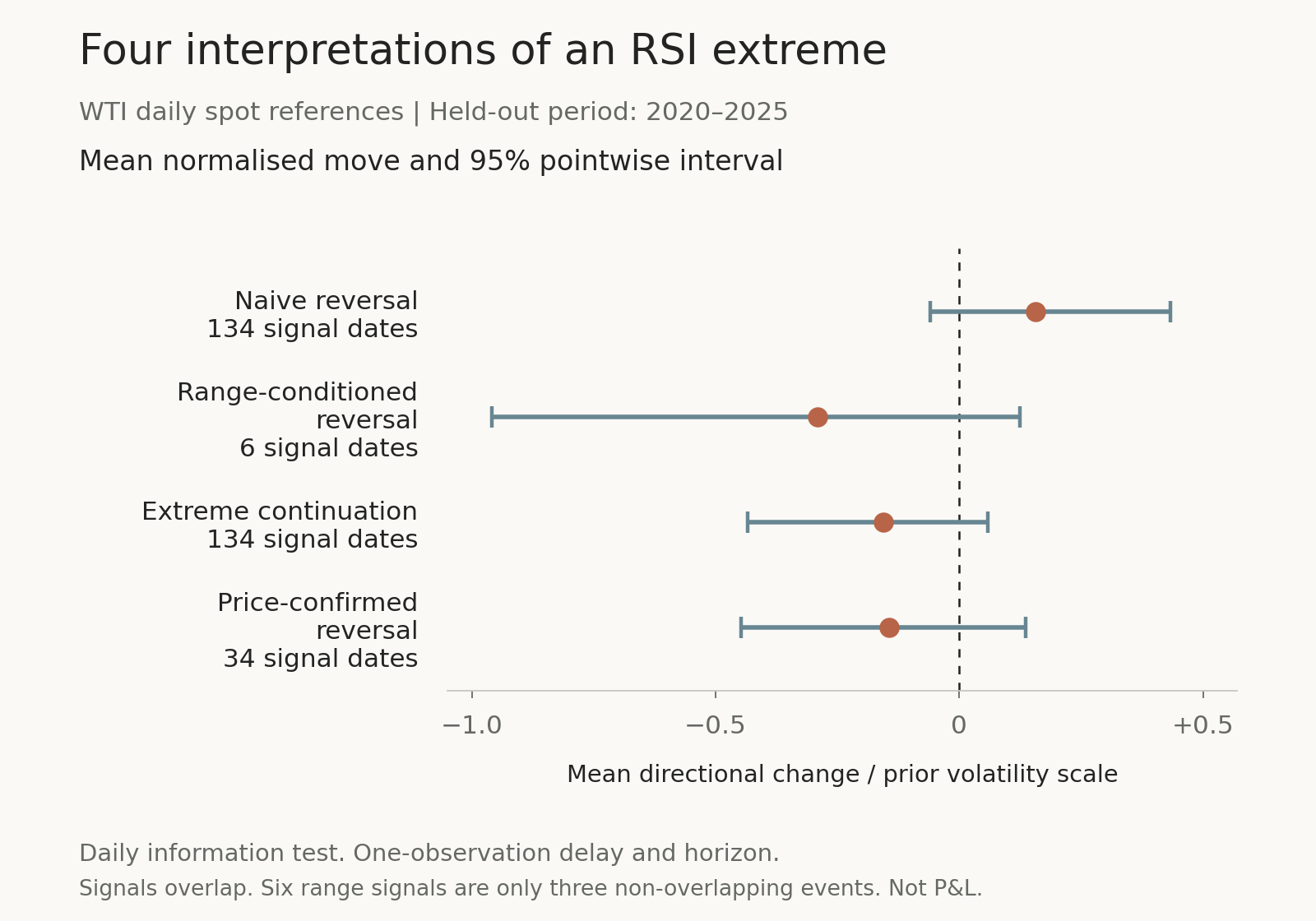
Figure 2. Newly tested daily-reference information results, WTI, 2020–2025. Dots show mean directional price changes divided by the rolling 20-observation standard deviation of price changes. Bars show 95% pointwise block-bootstrap intervals. One-observation delay and horizon. Counts are signal dates, not independent trades. These are not returns or net trading profits. Source: the project's saved calculations from EIA observations.
The naive WTI reversal rule produced 134 extreme signal dates at the one-observation horizon. Its average normalised move was +0.156, with a 95% pointwise interval from −0.059 to +0.434. That uncertainty includes negative values. Nearby parameter choices and longer reference delays changed the result, including its sign.
The range-conditioned version retained only six of those 134 dates. Under the study's non-overlap scheduling rule, those six became just three reference events. It would be unreasonable to crown that filter, or condemn it universally, from such a small sample.
Among 43 separately identified WTI extreme episodes, 28 received the defined price confirmation within five observations. Median confirmation delay was three observations. Some favourable reversals occurred without confirmation. Episode windows could overlap, so these were not 43 independent experiments. The lesson is modest but useful: confirmation changes timing and selection, and those changes have costs as well as possible benefits.
Adding RSI, EMA slope and volatility context did not establish a robust improvement over the price baseline. For one-observation WTI direction forecasts, Brier loss was approximately 0.251687 for the full model and 0.251084 for the price baseline. Lower is better: Brier loss measures squared error between forecast probabilities and actual binary outcomes.
One narrow EMA-only comparison improved on that price baseline after adjustment for multiple comparisons, with some numerical uncertainty near the rejection threshold. But EMA-only still scored worse than the constant training-frequency forecast: 0.249549 versus 0.249441. “Better than this baseline” was not the same as “better than the simplest available forecast.”
The analysis accounted for 630 final model comparisons across instruments, horizons, benchmarks, ablations and bootstrap-block variants. No component-removal result survived that family adjustment as evidence for keeping a component. This is evidence about these specified daily models, not a proof that every possible use of an indicator is futile.
For actual intraday CL, the accessible Portara/CQG named-contract sample contained only 74 complete 15-minute bars from one partial session. That was enough to check calculations and bar timing. It was nowhere near enough to establish an economic edge. No intraday MCX strategy, genuine order-flow strategy, profile strategy or options-profitability test was completed.
Richer data must earn its place too
VWAP and volume profile often feel more substantial than oscillators because they refer to where activity occurred. That can be useful, but it still leaves a forecasting question.
Suppose three hypothetical trades occur: two contracts at 80, one at 81, and three at 79. Exact trade VWAP is (2×80 + 1×81 + 3×79)/6 = 79.67. Price above that reference means price is above the volume-weighted mean of those trades. It does not reveal all participants' entry prices, remaining positions or intentions.
A bar-based typical-price VWAP is an approximation to trade-level VWAP. An anchored VWAP also depends on when accumulation begins. An anchor chosen because a turning point looks obvious in hindsight is different from an anchor specified before the outcome.
A volume profile adds a distribution across price bins. The point of control (POC) identifies a maximum-volume bin; value-area high and low (VAH and VAL) bound a chosen value-area construction. Time-price opportunity (TPO) profiles instead count time-at-price opportunities. These are distinct measurements. Session boundaries, bin width and the availability of developing data change what can legitimately be known at a decision timestamp.
TradingView specifically documents that its volume-profile up/down split uses lower-timeframe bar direction. It is not exchange-reported aggressor buy/sell classification. A coloured profile cannot silently become a genuine trade-delta feed. TradingView's methodology
With suitable trade records, delta subtracts sell-aggressor volume from buy-aggressor volume. Cumulative volume delta (CVD) accumulates it. Every execution still has a buyer and seller; delta classifies which side sought immediate execution. Order-book-event imbalance additionally incorporates changes in displayed liquidity and is a different object.
Cont, Kukanov and Stoikov found a relationship between order-flow imbalance, market depth and short-interval price changes in their equity sample. Explaining price movement within an interval does not establish a forecast that can be traded after observing the interval, and it does not automatically transfer to CL.
Positive delta without upward price progress could motivate an absorption hypothesis. To make that useful, define the observation window, price tolerance, classification method and subsequent response in advance. Replenishing offers are one possible explanation. Misclassification, changing quotes or an arbitrary window are alternatives. “Institutional accumulation” is a claim about identity and intent that these observations do not establish.
Open interest, futures curves, implied volatility and skew can add context. Public open interest does not identify signed dealer inventory, so gamma exposure remains an estimate conditional on positioning assumptions. The companion article How Options Move Markets follows those distinctions in more detail.
A difficult market exposes the hidden assumption
Here, adversarial means conditions that defeat ordinary assumptions. No deliberate manipulation is required.
| Situation | Tempting inference | The assumption to challenge |
|---|---|---|
| Persistent trend | An extreme oscillator must reverse. | A recent imbalance has reached an economic limit. |
| Choppy range | The next moving-average crossover starts a trend. | A brief directional change will persist enough to cover costs. |
| False breakout | Crossing the level proves acceptance. | Other participants will keep transacting beyond it. |
| Abrupt repricing | The old range and usual stop distance remain useful. | Historical variation still describes current liquidity and uncertainty. |
| Conflicting flow | Positive delta guarantees higher prices. | Aggressive buying will overwhelm available and replenishing offers. |
| Moving profile | Yesterday's POC remains an enduring magnet. | The selected historical auction is still relevant. |
| Missing or delayed data | The displayed setup is actionable now. | The screen represents the market at the decision timestamp. |
These failures suggest four separate meanings of robustness. Computational robustness asks whether a calculation survives reasonable seed, sampling and missing-data choices. Parameter robustness asks whether nearby settings retain usefulness. Market robustness asks whether it survives different sessions, regimes, instruments and structural changes. Economic robustness asks whether an explicit decision still has value after spreads, fees, slippage, latency and realistic fills.
An indicator may pass the first test and fail the other three. Smoothness should never stand in for all four.

Figure 3. Conceptual illustration. A continuation story and a reversal story can both remain plausible. Original generated artwork, not a forecast or historical price path.
Two measurement blocks and a decision gate
The smallest defensible interpretation framework emerging from this work has three parts. Its inclusion standard is functional usefulness with known limits, not proven trading alpha.
First, causal price structure. Record where price is relative to references that existed at the time: the previous completed session's high and low, lagged range boundaries, and pivots only after their required confirmation. One simple direction descriptor, such as an EMA slope, can make an informal label reproducible. It does not need a second and third oscillator to repeat the same message.
Second, one volatility scale. Use ATR with valid OHLC data, or a specified return or price-change volatility estimate with appropriate inputs. Ask how extended the movement is and how plausible adverse scenarios compare with recent variation. Treat jumps, liquidity gaps and loss limits separately. A volatility multiple does not guarantee a fill or contain tail risk.
Third, a decision gate. Confirm the contract, clock, feed quality, event timing and execution assumptions. If spreads or uncertainty overwhelm the advantage independently established for the rule, abstain. If no such advantage has been established, the framework remains an interpretation exercise.
Volume and order flow are optional additions only when reliable data and a defined use justify them. If buying and selling pressure cannot be observed, write unknown. Completeness does not require an invented answer in every box.
Building a story that can be wrong
Consider a fictional CL example, not a current market assessment.
The completed one-hour bars show a declining sequence of closes. On the 15-minute chart, price is below the previous completed session's low of 78.40. RSI is 24. Recent attempts to recover the level have failed. Assume ATR14 is 0.45. Genuine classified trades and depth are unavailable.
The observation supports a cautious primary hypothesis: downward persistence remains the working explanation. The RSI reading describes that recent imbalance; it does not independently prove exhaustion. The strongest alternative is a failed breakdown followed by a recovery into the old range.
Now make the distinction observable. An illustrative reversal condition might require two completed 15-minute closes above 78.40, followed by a separately defined five-minute pullback that holds that level. Those conditions are examples to test, not optimised or validated rules. They would delay entry, and some rebounds would occur without satisfying them.
If price instead makes fresh lows and cannot reclaim the reference, the continuation account remains more consistent with the observed behaviour. If price regains the range and holds it, the initial account needs revision. If an inventory announcement produces a gap, stale quotes or sharply wider spreads, the original execution assumptions may no longer apply at all.
The sequence is context → location → observed behaviour → available participation evidence → price response → competing hypotheses → confirmation and invalidation → risk.
This is a way to update an explanation. It is not a bullish/bearish vote count. The broader distinction between a market thesis and its path is explored in Why Bullish Oil Markets Still Pull Back.
Taking the question from CL to MCX
The transfer needs its own evidence. CL is quoted in dollars per barrel; MCX crude is quoted in rupees per barrel. Currency movement, contract matching, basis, local sessions and liquidity can change the relationship. A CL level multiplied by USD/INR is a useful starting reference under stated assumptions, not a guaranteed live MCX execution price. Use the applicable MCX contract specifications and CME CL rules, including the actual contract month.
Likewise, a correct underlying forecast does not establish a profitable option purchase. Premium responds to implied volatility, time, convexity and the executable bid-ask spread. An option can lose despite a favourable underlying move. The forecast and the instrument used to express it need separate evaluations.
For research, a 15-minute decision chart can be paired with completed one-hour, four-hour and daily context, and five-minute execution observations. These are different views of overlapping data, not independent witnesses. A signal calculated at a bar close must be evaluated using a feasible later execution opportunity. A delayed research feed cannot establish a current entry on a faster timeframe.
What would change the conclusion?
A richer framework could earn inclusion. It would need a clean, timestamped, contract-level CL or MCX dataset and a decision rule specified before examining the final test period. It should beat the strongest simpler alternative after conservative execution costs, not merely a weak benchmark.
The tests would need nearby parameters, difficult sessions, event windows, delays, gaps, turnover, drawdowns and missed opportunities. Removing each component should reveal whether it contributes anything after the others are present. All tried filters, settings and combinations belong in the search history. Overlapping outcomes require dependence-aware uncertainty; repeatedly inspecting a supposed holdout makes it part of development.
A result that survives those challenges would change the assessment. Failure should change it too. The useful objective is a process that can reject an attractive idea.
A compact interpretation note
Before making a market claim, fill in the following in ordinary language:
Instrument, contract, timestamp and data quality:
Decision timeframe and completed higher-timeframe context:

Direction:
Buying/selling pressure, or unknown:
Trend strength and how it is measured:
Location relative to pre-existing levels:
Volatility and extension:
Continuation evidence:
Reversal evidence:
Contradictory evidence:

Primary hypothesis:
Strongest alternative:
Required confirmation and its timing cost:
Invalidation:
No-trade condition:

Confidence and its evidence:
What these data cannot tell me:
An answer such as “pressure unknown; price still below the prior range; reversal unconfirmed” can be more useful than a colourful set of signals that all reuse the same input.
The value of an indicator begins with knowing what it measures. The value of a market story depends on specifying what would make us change it.
Research and illustration notes
Research date: 20 September 2026. This is an educational synthesis of a targeted literature review and a limited original computational study, not a peer-reviewed validation of a trading system. The 81-candidate inventory was a broad definition and evidence screen; it was not 81 strategy backtests.
Daily features and model specifications were frozen before final holdout evaluation. Later increases in bootstrap precision were documented and did not change model forecasts. The daily data were not a point-in-time publication archive. Some outcomes and episodes overlap, and sparse conditional samples limit interpretation. No purchase, subscription, trade, genuine footprint reconstruction or options-P&L backtest was made.
The cover and two conceptual illustrations were generated for this article in the journal's ivory, terracotta, charcoal and muted-blue palette. Figure 2 was rendered directly from saved numerical results. Its uncertainty bars are pointwise estimates, not a multiple-testing-adjusted ranking of the four RSI rules. Hypothetical arithmetic and the fictional market story are labelled where they appear.