
Cover: an original conceptual illustration of direction and retracement. This essay uses dated historical evidence, not a forecast for September 2026.
Imagine WTI climbing from $90 to $100 after a supply shock. The threat to supply remains. Inventories still look tight. Then oil falls to $96.
Those prices are hypothetical, but the question is familiar: if the case for higher oil prices survives, why would anyone sell?
The question quietly assumes that a bullish belief requires continuous buying. It does not. A producer may want to secure an attractive selling price. A fund may need to reduce risk. A buyer who was enthusiastic at $90 may see little advantage at $100. Another trader may think the disruption will be shorter than the market previously feared.
A bullish thesis is a view about a distribution of future outcomes. It is not a promise about the next transaction.
I find it useful to separate the case for owning an exposure from the conditions under which that exposure changes hands. Fundamentals, expectations, liquidity and trading constraints interact. None gives us a guaranteed route to a destination.
The news still has to meet an auction
In Albert Kyle’s 1985 model, market makers observe aggregate order flow without being able to separate an informed trader’s orders from noise trading. They adjust prices as they learn from that flow. The contribution is a mechanism connecting information, trading and price discovery, not a formula for predicting WTI.
In an electronic order book, a buyer seeking immediate execution accepts available offers. If the order exhausts the quantity at the best offer, further execution must reach higher offers. A seller seeking immediacy does the reverse, trading against bids.
Every completed trade has a buyer and a seller. “Buying pressure” describes the urgency and price concessions of the initiating side relative to available liquidity, not a numerical excess of buyers over sellers.
Nor must every price revision wait for a trade. After news, participants can cancel orders and change quotes before anyone executes. The book itself is part of the response.
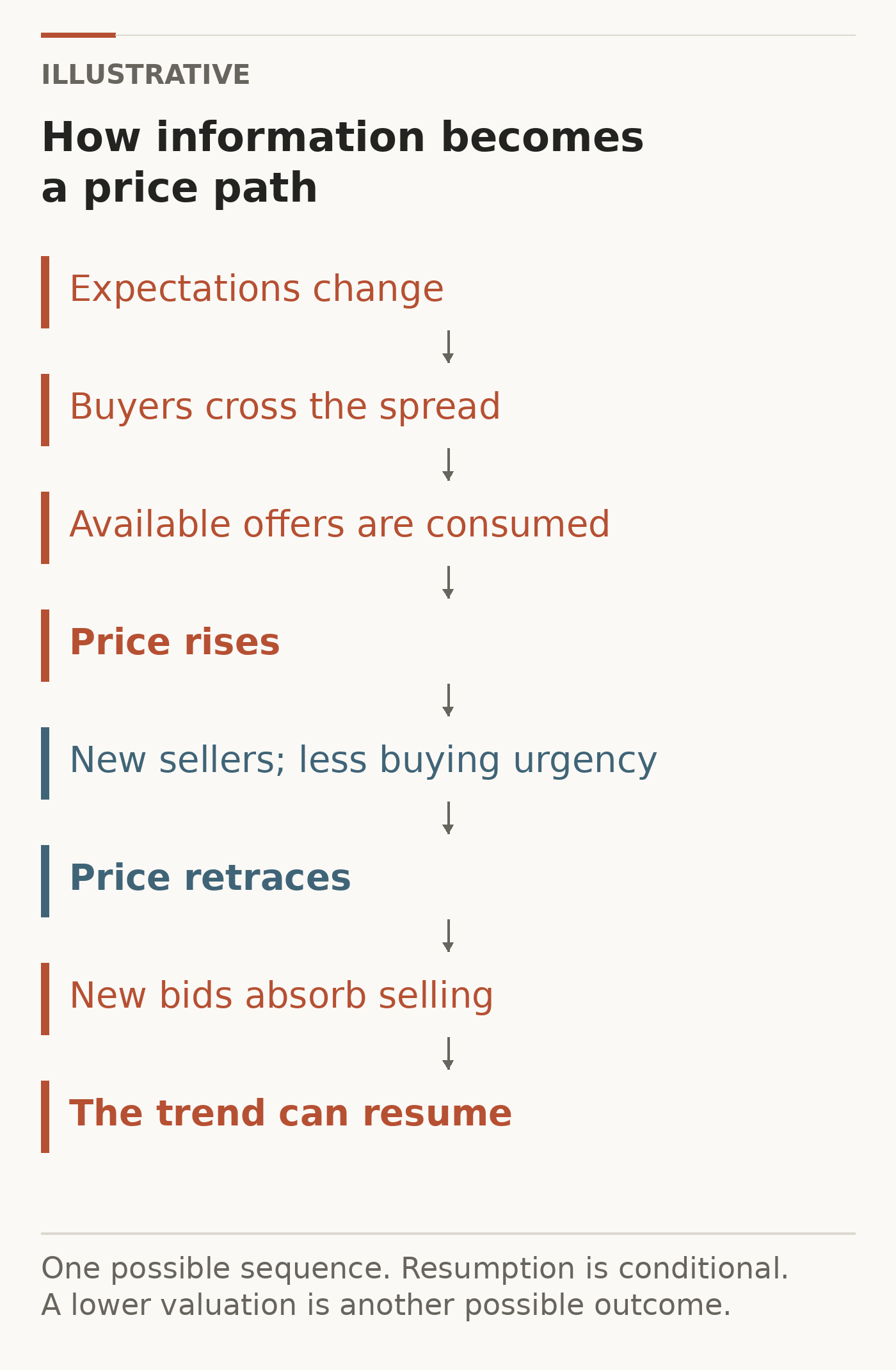
Figure 1. Illustrative mechanism, with no historical time range. Information can generate a rise, a retracement and a renewed advance, but the final step is conditional. Conceptual synthesis informed by Kyle (1985) and Grossman and Miller (1988).
Joel Hasbrouck’s 1991 research models trades and quote revisions jointly, using their eventual price effect to measure information content. In his stock-market sample, the full effect need not arrive immediately. That distinction helps us ask whether a move reflects lasting information or a more temporary trading disturbance. The study does not establish which explanation applies to a particular oil sell-off.
Grossman and Miller supply another piece: liquidity is a service of immediacy. Intermediaries bear risk between the arrival of ultimate buyers and sellers. Their willingness to do so has a price.
Inventory models make this concrete. A liquidity provider already carrying an unwanted position has a reason to change its quotes. Olivier Guéant’s synthesis of market-making models describes that interaction between inventory risk and quote placement. These are mechanisms we can apply cautiously to oil’s auction, not oil-specific measurements of their size.
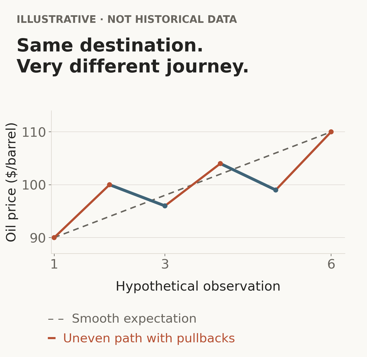
Figure 2. Illustrative, not historical data. The six observations have no assigned dates. Both invented paths end at $110; the intermediate risk is very different. Source: author-created teaching example.
Even observable selling does not reveal its motive. On 4 December 2024, Reuters reported a large WTI block trade and a rapid price decline. CME confirmed the block’s size, while the reported bank involvement and subsequent resale came from an unnamed source. That episode illustrates the limits of knowing why an order appeared, rather than proving a general explanation for pullbacks.
A historical example that complicates the story
The first half of 2022 is useful because the supply concern was documented at the time. We do not have to invent a bullish narrative after seeing the chart.
On 16 March, the IEA’s Oil Market Report described the risk of a major Russian supply disruption following the invasion of Ukraine. It also reported depleted OECD industry inventories. But the same report reduced its demand outlook and described economic concerns, Covid cases in China and position reductions amid extreme volatility. Supply risk had not disappeared; other inputs were moving.
The EIA’s daily Cushing WTI spot series fell from $123.64 on 8 March to $94.85 on 16 March: a $28.79 decline, or 23.3%. It subsequently reached $116.20 on 25 March, fell to $94.22 on 11 April, and recovered to $121.94 on 8 June. The second decline was 18.9%; the April-to-June recovery was 29.4%.
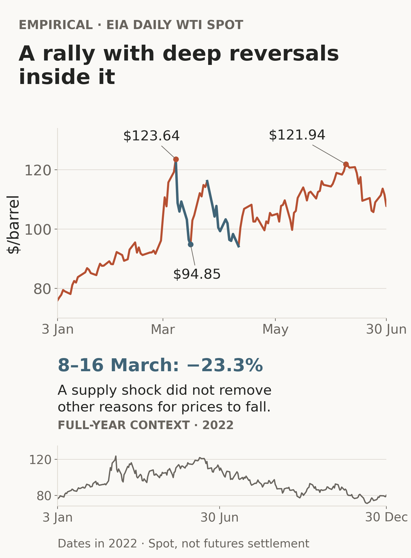
Figure 3. Empirical. Upper panel: 3 January–30 June 2022. Lower panel: 3 January–30 December 2022. Source: EIA, Cushing WTI spot price FOB, daily, dollars per barrel. Calculations use the named daily observations, not intraday extremes. Lines connect available observations; missing dates are not filled. These are spot prices, not a continuous futures contract or CME settlements.
This is a selected historical illustration, not a representative sample or an estimate of how often pullbacks recover. The fixed half-year window includes the June retreat, and the full-year context shows that the broader advance did not last indefinitely.
Most importantly, these prices cannot isolate profit-taking, liquidation, changing demand expectations or any other cause. The episode supports a narrower conclusion: severe retracements can coexist with a documented supply threat and a subsequent recovery. It does not establish that every fundamental input stayed unchanged.
The same bullish trader can rationally sell
A fund can keep its six-month oil view and reduce its position today. Perhaps the rally made oil too large a share of the portfolio. Perhaps higher volatility increased measured risk. Perhaps losses elsewhere created a need for cash.
Consider a deliberately simplified position-sizing rule: exposure equals a fixed risk budget divided by estimated volatility. If estimated volatility doubles, that rule halves exposure, even when the directional signal remains positive. This is arithmetic under an assumed rule, not a claim about every fund’s behaviour. Value-at-Risk limits and portfolio correlations can make the real calculation more complicated.
Profit-taking is another possibility, but it should not become a label attached to every unexplained red candle. It is a hypothesis about motives until supported by position or flow evidence.
Shleifer and Vishny’s The Limits of Arbitrage explains why conviction and staying power can diverge. Investors may withdraw money after a manager’s losses, just when an apparent mispricing becomes larger. The capital available to express a view can shrink while that view remains attractive to the manager.
An outright oil position is not the arbitrage trade in that paper. The transferable lesson concerns financing and delegated capital.
Selling is an action. Bearishness is a belief. The two do not map one-to-one.
A producer has something different to protect
For an oil producer, rising futures prices may make a hedge attractive because they improve the cash flow that can be secured. Selling futures offsets some of the producer’s existing exposure to the oil it expects to sell. The EIA explicitly distinguishes that producer hedge from an oil consumer’s purchase of futures.
A producer selling a suitable futures contract at $100 need not expect $80 later. It may prefer greater certainty over the possibility of $120.
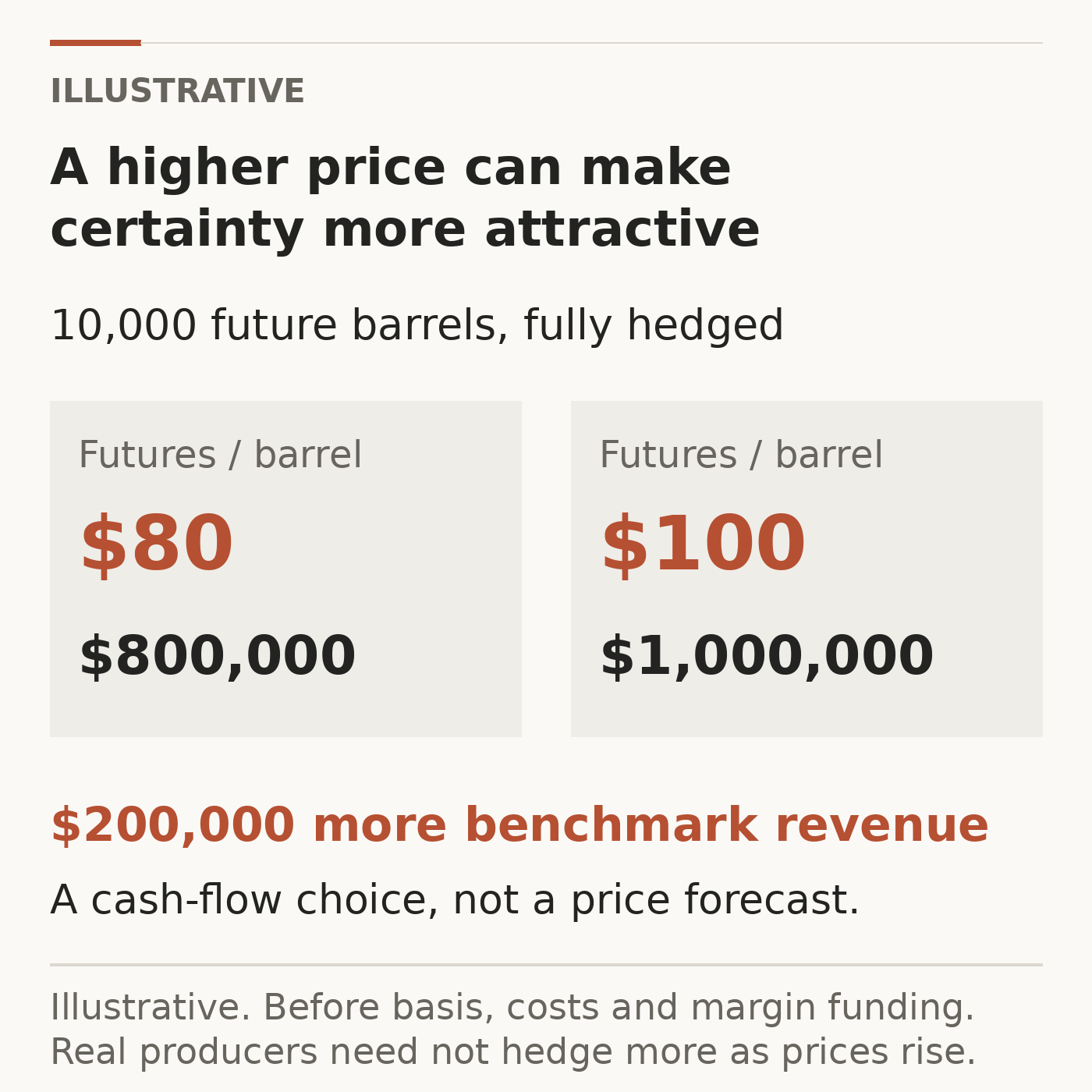
Figure 4. Illustrative hedge arithmetic, not an observed producer response curve; no historical dates. The $200,000 difference is 10,000 barrels × $20. These are benchmark revenues, not profits. Concept informed by the EIA’s explanation of oil-market hedging.
In the simplest matched hedge, the physical selling price plus the futures gain or loss approximates the initial futures price. In practice, location and quality differences, contract timing, production uncertainty, costs and margin funding remain relevant. A high front-month quote also does not mean a producer can lock that price for delivery much later.
There is oil-specific research behind the broader risk-transfer argument. Acharya, Lochstoer and Ramadorai, published in the Journal of Financial Economics in 2013, examine energy markets and producer hedging. Their model and evidence connect hedging demand, constrained speculative capital and futures risk premiums. If fewer investors can absorb the risk producers want to transfer, the price of that transfer changes.
This does not demonstrate a universal rule that a higher oil price produces more hedge selling. Existing hedges, balance sheets, management policy and the forward curve can change the response. The paper itself notes limitations in using aggregate hedging pressure to forecast returns.
Also separate two meanings of “risk premium”. Compensation for bearing futures risk is not the same concept as the extra price associated with a feared geopolitical disruption. They can interact, but they are not interchangeable measurements.
Good news is measured against expectations
Suppose traders had already positioned for a prolonged supply interruption. Confirmation that some supply is disrupted can still disappoint that expectation if the interruption now appears smaller or shorter.
The news is supportive compared with an undisturbed world, yet less supportive than the scenario embedded in yesterday’s price. There is no contradiction in prices falling.
This is the useful part of “buy the rumour, sell the fact”. The phrase describes a possibility, not a law. The harder task is reconstructing what was expected beforehand, using dated forecasts and evidence rather than claiming, after the event, that the outcome was “priced in”.
A supply shock also changes several questions at once. How many barrels are threatened? For how long? Can buyers substitute? Will governments release reserves? Will higher costs weaken demand? The March 2022 IEA report is a concrete example of supply concerns and demand downgrades appearing together.
Uncertainty can therefore expand while the expected price remains elevated. That does not mean bullish markets must be more volatile. It means a stronger average outlook can coexist with a wider range of plausible outcomes, which is quite different from a smooth upward path.
Less buying can matter as much as more selling
When an urgent buyer finishes, another buyer does not automatically take its place at the same price. If sellers are still willing to trade immediately, the next transaction may occur lower.
The depth available at those lower prices matters. A modest order can move through several levels in a thin book, while a larger order may have little impact against deep, replenishing liquidity. Displayed quantity is only a snapshot: orders can disappear, new orders can arrive, and some liquidity is not displayed.
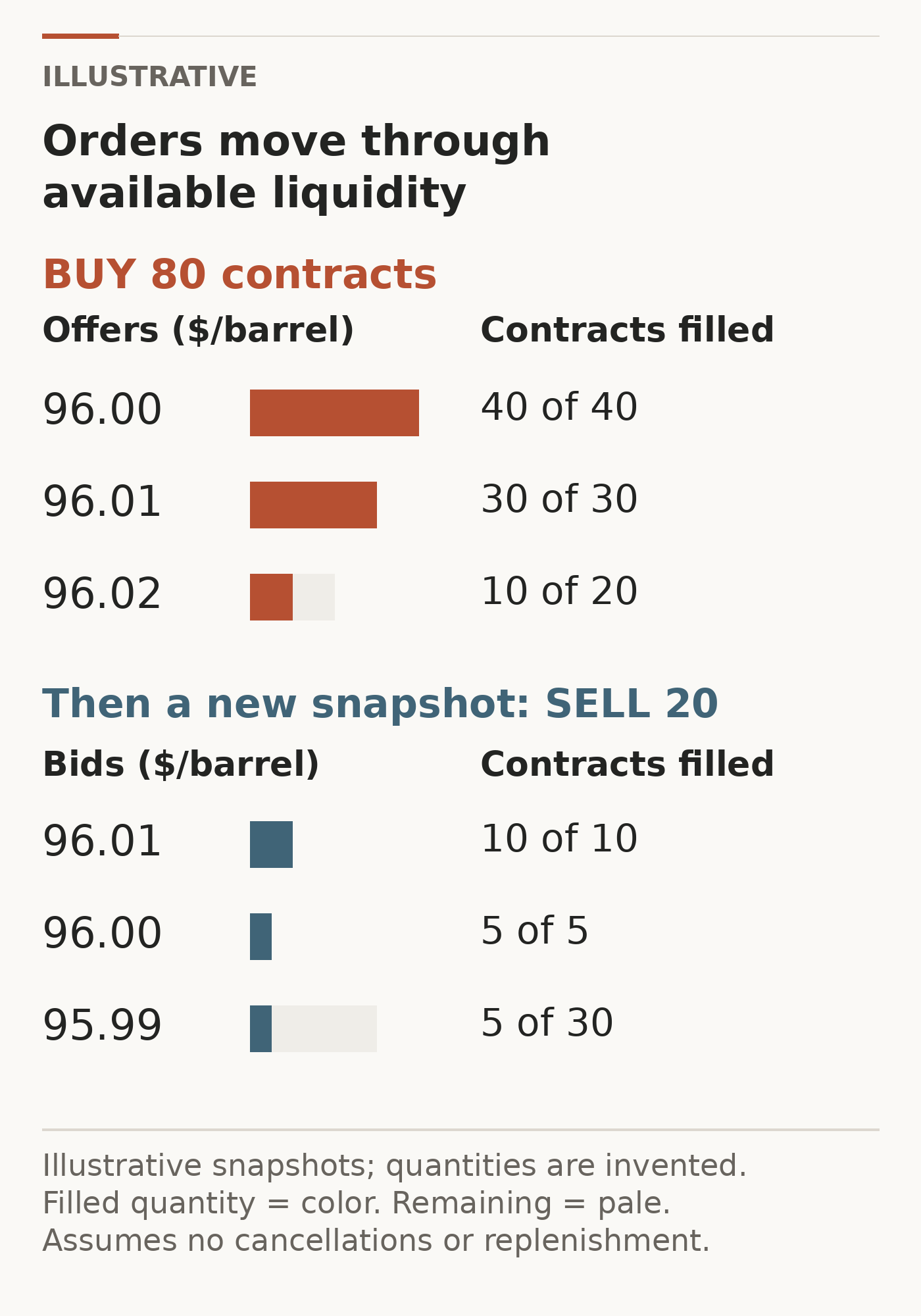
Figure 5. Illustrative execution accounting; quantities and snapshots are invented, with no historical dates. Prices are dollars per barrel, quantities are contracts. The example holds each snapshot fixed while its order executes. This isolates the mechanism discussed in market-making research, not the complexity of a live WTI book.
Notice what this example does not establish. It does not identify the traders, reveal their beliefs or measure a lasting change in value. A trade record tells us what happened at the auction. Explaining why requires more evidence.
Leverage can turn a retreat into a feedback loop
An ordinary decline becomes more consequential when participants cannot finance it. Falling prices create losses for leveraged longs. Some reduce positions to meet margin calls or risk limits. Their sales may hit an already thin book, producing larger losses for others.
Stop orders can contribute too, although a triggered stop is not necessarily a forced liquidation. One follows a pre-set exit instruction; the other reflects a financing or risk constraint. Nor does a stop guarantee execution at its trigger price.
Brunnermeier and Pedersen’s Market Liquidity and Funding Liquidity formalises feedback between the ability to finance positions and the ability to trade them. Losses and, under particular conditions, higher margins can reinforce illiquidity. Their model is a reason to investigate amplification, not permission to call every decline a liquidation cascade.
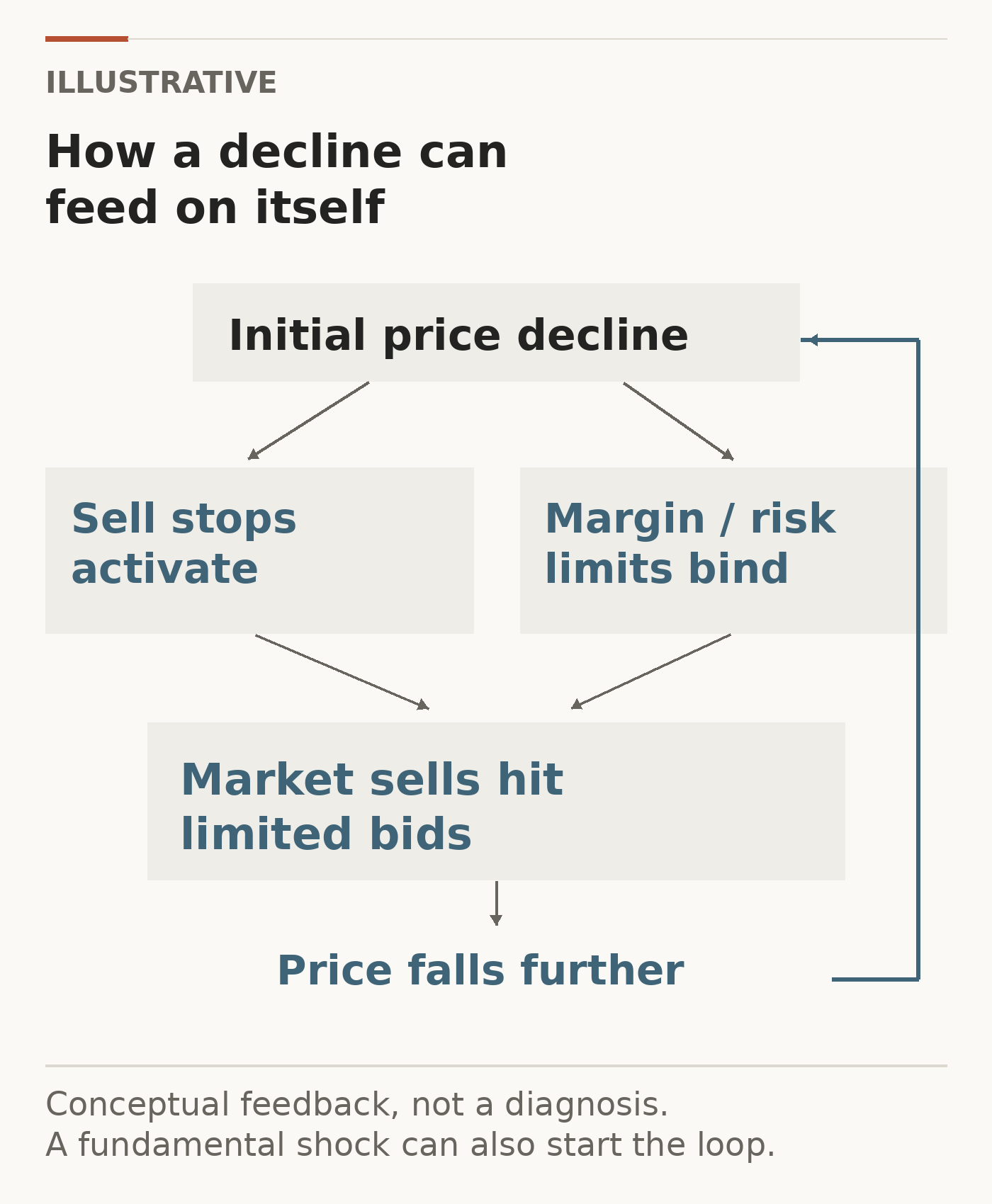
Figure 6. Conceptual feedback loop, not an observed liquidation sequence. No historical time range. Source: author synthesis informed by Brunnermeier and Pedersen (2009). A fundamental shock can also initiate or accompany the loop.
Size makes the path matter. The standard CME WTI futures contract represents 1,000 barrels. A hypothetical $4 adverse move therefore means $4,000 per contract before trading costs. A trader can be correct about a later recovery and still be unable to hold through that loss.
Options can change the direction of hedging
Delta measures an option’s price sensitivity; gamma describes how delta changes as the underlying moves. For an option on futures, the relevant underlying is its futures contract.
Take an illustrative dealer holding 100 calls with delta 0.50 per call. The option position has about 50 futures contracts of directional exposure. Selling 50 matching futures approximately neutralises it. If price rises and delta becomes 0.60, the dealer sells another 10 futures to restore neutrality. That is a positive-gamma book selling into a rise.
Reverse the option position. A dealer short those calls initially buys 50 futures. When delta rises to 0.60, it must buy 10 more to rebalance. That is a negative-gamma book buying into a rise. On a decline, the corresponding hedge directions reverse.
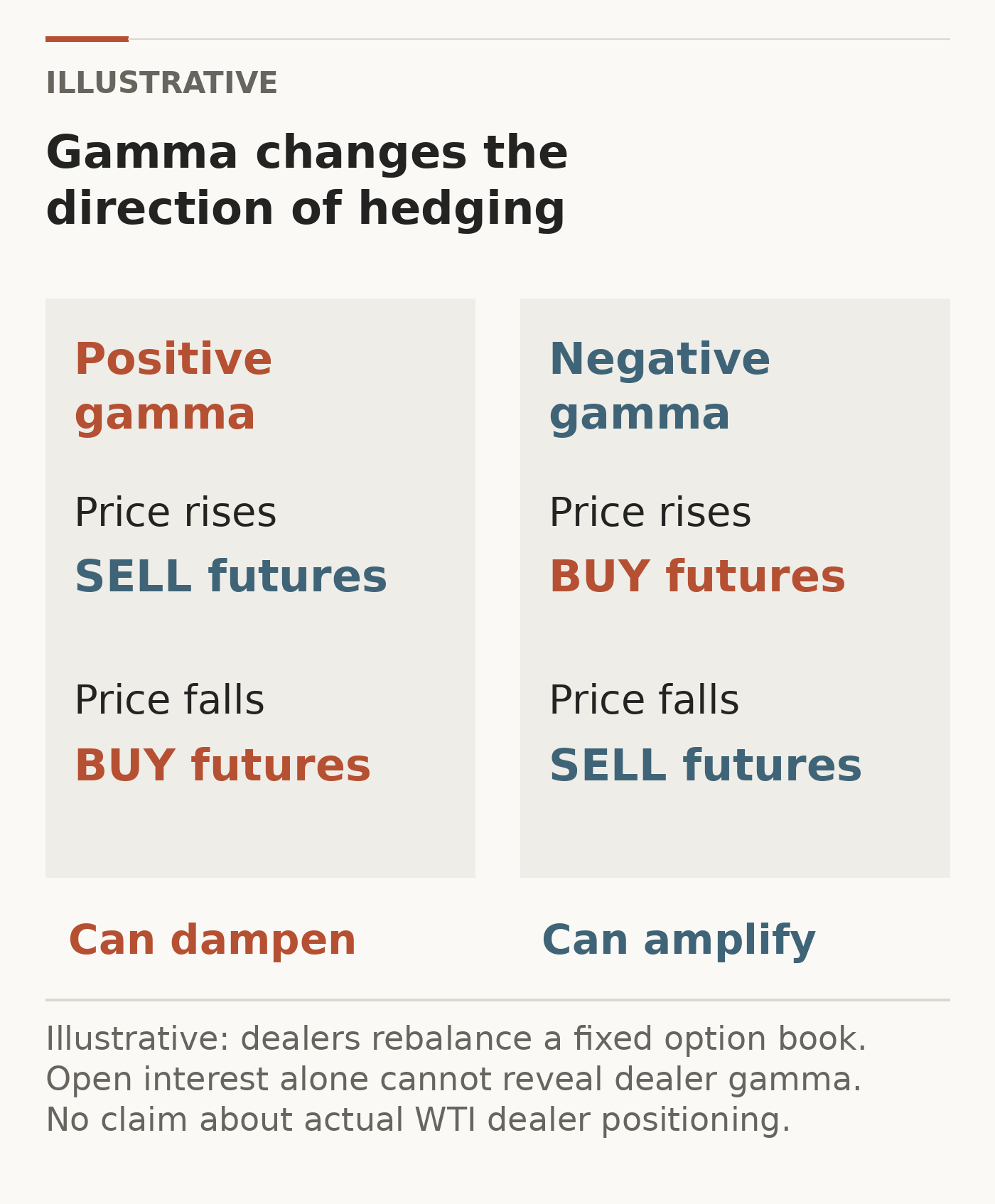
Figure 7. Illustrative options mechanics, not an estimate of WTI dealer exposure; no historical dates. Source: hedge arithmetic using CME’s gamma definition. The book, time and volatility are held otherwise unchanged. Open interest alone cannot reveal dealer gamma.
Positive gamma can therefore add trading against a move; negative gamma can add trading with it. Whether that meaningfully dampens or amplifies the market depends on exposure, rebalancing and available liquidity. Other flows can overwhelm it.
The distinction applies to the dealer’s net book, not to “calls versus puts”. Long conventional calls and puts both have positive gamma; short positions reverse that sign. Volatility changes, time passing, new trades and hedges in other instruments further complicate the flows.
Keep three levels separate: the mechanics are established; a vendor’s exposure map is a model estimate; an explanation of a particular WTI move is a hypothesis requiring evidence. Open interest counts outstanding contracts, each with a long and a short. It does not tell us which side dealers own, nor their offsetting positions. This essay has no defensible dealer inventory dataset and makes no claim that dealers caused the historical retracements.
One market contains several different clocks
A producer may plan cash flow over months. A macro fund may evaluate a multi-month supply deficit. A swing trader may work over days, while an intraday trader wants a move to finish before the session ends. Market makers continually manage execution and inventory risk.
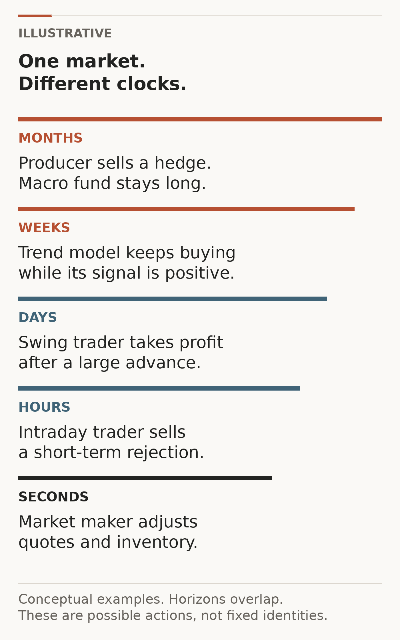
Figure 8. Conceptual participant map, not measured holding periods or fixed classifications. No historical time range. Sources: EIA’s participant overview, market-making research and Moskowitz, Ooi and Pedersen’s momentum research.
Moskowitz, Ooi and Pedersen document time-series momentum across futures markets, including commodities. This supports studying systematic trend strategies as a distinct form of participation. It does not reveal today’s CTA positions, imply all CTAs follow the same model, or identify a price where they will trade. A price-trend model can stay long while a volatility overlay reduces its size.
Opposite transactions can thus be rational responses to different objectives. They need not all prove profitable. What disappears is the apparent inconsistency in a longer-term bull and a shorter-term seller sharing the same market.
How much should a pullback change the thesis?
I would start with a more demanding question than “Was the headline bullish?”: Compared with the prior expectation, what changed, and how did the market respond?
Repeated failure to advance after genuinely positive surprises deserves investigation. So does selling that persists despite apparently supportive information. Neither proves the cause. Expectations may have been wrong, positioning crowded, liquidity poor, or the physical picture weaker than assumed.
The tools below answer different questions. Combining them is useful; treating several related price indicators as independent confirmation is less convincing.
| Evidence | What it can help assess | What it cannot establish |
|---|---|---|
| VWAP and market structure | Trading relative to a volume-weighted benchmark; whether breaks and rebounds persist on the chosen timeframe | Fair value or why a participant traded. The session, anchor and horizon matter. |
| Volume profile and traded volume | Where and how much business occurred over the selected interval | Future support, fresh buying intent or trader identity. Every trade has two sides. |
| Trade delta | Aggressive buy-initiated versus sell-initiated volume, when the feed supports that classification | Total bullishness or hidden inventory. Candle-based estimates are not direct aggressor records. |
| Futures open interest | Whether outstanding contracts expanded or contracted | “New shorts” or “long liquidation” by itself. Opening and closing trades have counterparties; expiry and rolls matter. |
| CFTC positioning | Broad changes in reported participant exposures | An intraday trigger, a trader’s exact motive, or dealer gamma. |
| Options and volatility | The price of protection and the range of outcomes being valued | Dealer hedge direction from unsigned open interest, or a certain price target. |
| Inventories, spreads and physical differentials | Whether evidence of physical tightness strengthens or weakens | A complete global balance from one weekly number or one delivery location. |
For data definitions, see CME on open interest, the CFTC’s report guide, and TradingView’s documentation of its estimated cumulative volume delta. Indicator implementations and feeds matter.
The disaggregated CFTC report separates Producer/Merchant/Processor/User, Swap Dealers, Managed Money and Other Reportables, with nonreportable positions outside those reported groups. It ordinarily describes Tuesday positions released on Friday. The categories reflect participants’ predominant business, not the motive for each trade. A commercial classification does not certify that every position is a hedge. Futures-only and futures-and-options-combined reports also have different construction; the latter uses delta-adjusted options. The CFTC’s report guide and disaggregated explanatory notes explain these distinctions.
For physical evidence, the EIA treats inventories as both a buffer and a signal of the supply-demand balance. Read changes with seasonal patterns, refinery activity, trade flows and geography. A crude draw caused by stronger refinery runs has a different interpretation from one caused by interrupted imports.
Term structure adds another view. When nearby oil is more expensive than later delivery, backwardation can be consistent with immediate scarcity. But storage economics, financing and the benefit of having physical inventory available also matter. A curve is not an unbiased price forecast, and one calendar spread is not the entire thesis. CME’s explanation of contango, backwardation and convenience yield provides the basic framework.
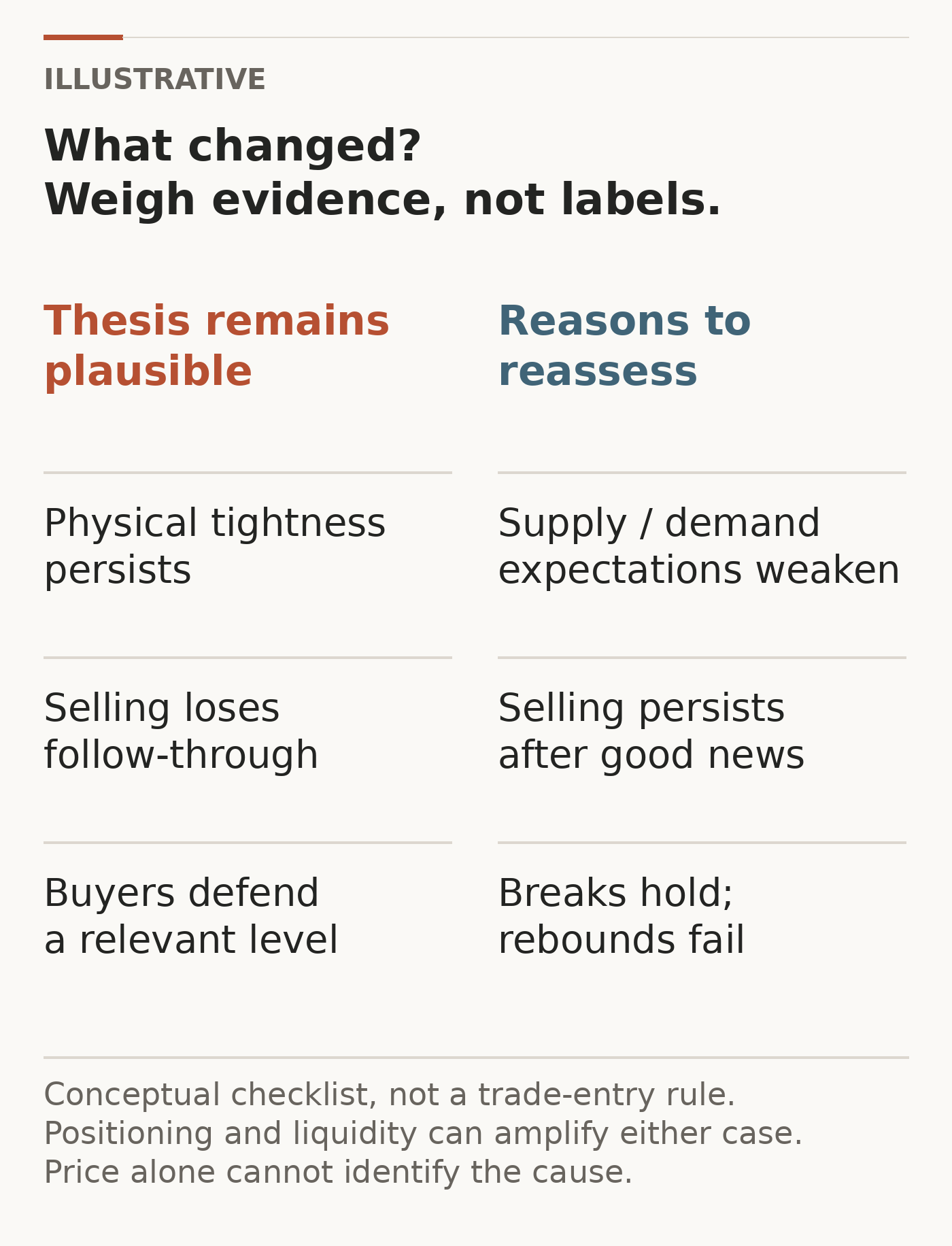
Figure 9. Conceptual diagnostic framework, not a validated signal or probability model. No historical time range. Source: author synthesis of the research above. Positioning and liquidity can amplify either case, so the columns are not mutually exclusive explanations.
The practical task is to revisit the proposition itself. Which supply or demand assumption justified it? What new evidence would weaken that assumption? Is the price action consistent with temporary risk transfer, or is the market persistently valuing a different future?
Physical balances, expectations, geopolitical uncertainty, financing and order flow are useful lenses. They are not independent dollar amounts that can simply be added into an “oil price equation”. The channels overlap: a physical shock can alter expectations, margins, hedges and available liquidity together.
A pullback tells us that sellers temporarily won an auction. It does not, by itself, tell us why they sold or whether the larger thesis changed. Finding out which part changed is the work. Calling the move “healthy” is a conclusion to earn, not reassurance to start with.
Sources and further reading
- Albert S. Kyle (1985), Continuous Auctions and Insider Trading, Econometrica 53(6), 1315–1336. Information revealed through order flow.
- Joel Hasbrouck (1991), Measuring the Information Content of Stock Trades, Journal of Finance 46(1), 179–207. Trades, quotes and eventual price impact.
- Sanford J. Grossman and Merton H. Miller (1988), Liquidity and Market Structure, Journal of Finance 43(3), 617–633. Immediacy and intermediary risk-bearing.
- Andrei Shleifer and Robert W. Vishny (1997), The Limits of Arbitrage, Journal of Finance 52(1), 35–55. Why capital constraints can limit conviction trades.
- Markus K. Brunnermeier and Lasse Heje Pedersen (2009), Market Liquidity and Funding Liquidity, Review of Financial Studies 22(6), 2201–2238. Margin and loss feedback.
- Viral V. Acharya, Lars A. Lochstoer and Tarun Ramadorai (2013), Limits to Arbitrage and Hedging: Evidence from Commodity Markets, Journal of Financial Economics 109(2), 441–465; accessible May 2012 manuscript. Energy-market evidence on hedging and constrained risk-bearing.
- Tobias J. Moskowitz, Yao Hua Ooi and Lasse Heje Pedersen (2012), Time Series Momentum, Journal of Financial Economics 104(2), 228–250. Systematic trend evidence across futures markets.
- Olivier Guéant (2016, revised 2017), Optimal Market Making, arXiv:1605.01862. Inventory-sensitive quoting models.
- IEA (16 March 2022), Oil Market Report. Contemporaneous supply, inventory and demand context.
- EIA, daily WTI spot observations, financial-market mechanisms, and inventory balances. Data and definitions accessed 12 September 2026.
- CFTC, Commitments of Traders and disaggregated explanatory notes; CME, gamma, open interest, WTI contract specifications, and futures supply and demand. Definitions accessed 12 September 2026.
- Reuters (4 December 2024), Bank sold over $270 million of US oil futures ahead of OPEC+ meet, source says. A bounded example of observable transactions and uncertain motives.
Data note: the empirical figure uses 251 published daily observations during calendar 2022. Nine weekday blanks are retained as missing in the accompanying data. Percent changes equal (later price ÷ earlier price − 1) × 100. All other figures are expressly illustrative. Neither the historical example nor the diagnostic framework estimates the probability of a profitable trade.