
Figure 1. Conceptual illustration. An option creates a choice; managing the resulting exposure can create feedback. Original generated artwork, not a price chart or a forecast.
Imagine buying a call because you expect an asset to rise. It rises. Your option loses money.
Now imagine seeing a large call purchase on an options feed. The label says “bullish”. Yet the buyer may be reducing an existing short position, protecting another exposure, or buying one leg of a larger trade.
Neither situation requires the market to be irrational. Both require us to ask a more complete question.
An option is a contract whose value depends on more than direction. Its owner and writer acquire changing exposures. Some participants manage those exposures by trading the underlying asset. Those hedge trades meet an auction with its own liquidity, competing orders, and constraints.
The useful chain is contract payoff → pricing inputs → Greeks → hedging → estimated exposure → observed flow → underlying liquidity. Each link answers a different question. Trouble starts when an estimate at one link is presented as a fact about the next.
Throughout this article, mechanics means a contractual or mathematical relationship; model estimate means an answer conditional on stated inputs; interpretation means a hypothesis about what participants might be doing. Our prices and positions are hypothetical unless an exchange specification is explicitly identified. Actual dealer inventory is unknown.
Contents
- 1. Options and obligations
- 2. Expiry payoff and earlier profit
- 3. Pricing inputs and executable quotes
- 4. Volatility and event risk
- 5. Delta, gamma, theta, vega and rho
- 6. Dealer inventory and hedge changes
- 7. GEX calculations and inventory assumptions
- 8. Transactions and options flow
- 9. Orders, liquidity and conditional scenarios
- 10. WTI and MCX contract mechanics
- A checklist for interpreting options data
- Reasoning questions and answers
- Glossary of key terms
- Technical notes and reproducible models
- Source directory
1. A right with a price
What exposure do you actually own?
Owning an asset gives you that asset's gains and losses. Buying a share at $100 and selling at $103 produces a $3 gain before costs. A futures contract instead creates a contractual exposure to a specified underlying and settlement date, generally with margin and daily settlement. A futures buyer cannot simply discard an unfavourable contract without settling or offsetting the position.
An option buyer pays for a right. A call gives a right to buy; a put gives a right to sell, under the contract's terms. The agreed price is the strike, the option's price is its premium, and its final date is its expiry. The writer, or seller opening a short option, receives premium in return for a corresponding obligation if assigned. OIC: options basics.
A reservation fee is a useful first analogy: you pay now to keep a choice available. A protective put resembles insurance against a fall in an asset you own. But exchange-traded options have standardised terms, tradeable prices, and specific settlement rules. A put can also be bought without owning the asset. It does not require a documented insurance loss or explain the buyer's entire portfolio.
Our running example is a fictional, non-dividend-paying equity near $100, with 100 shares per option contract. That multiplier is an explicit assumption, not a universal options rule. Premiums below are dollars per share unless stated otherwise. A $3.59 premium means about $359 for this assumed contract.
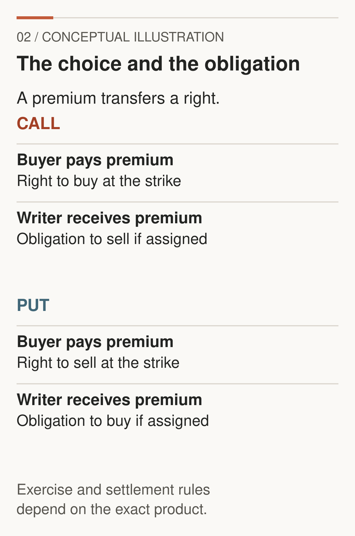
Figure 2. Conceptual illustration. The buyer purchases a right; the writer accepts an obligation. The exact exercise and settlement mechanics come from the product specification. Source: author diagram based on OIC's options basics.
There are four basic positions. “Long” means owning the option; “short” means having written it.
| Position | What it provides | Standalone risk in this equity example |
|---|---|---|
| Long call | Right to buy at the strike | Can lose the entire premium and costs; upside is theoretically unbounded |
| Short call | Obligation to sell if assigned | Premium is the maximum option profit; an uncovered call has theoretically unbounded loss |
| Long put | Right to sell at the strike | Can lose premium and costs; maximum expiry payoff occurs at a zero share price |
| Short put | Obligation to buy if assigned | Substantial loss as shares fall, up to strike × multiplier less premium, before costs |
These are standalone positions. A covered call combines a written call with the shares needed for delivery. That cover addresses the naked call's delivery exposure but leaves the stock's downside. An option spread can offset some risks with another option. “Hedged” describes a relationship between positions, not immunity from losses. OIC: long call, long put, and uncovered call.
Exercise uses the right. Assignment allocates the corresponding obligation to a writer through the clearing and broker process. Closing is different: a holder sells an equivalent option to close; a writer buys it back to close. Closing does not require finding the original counterparty. Assignment procedures and broker deadlines matter independently of the option's apparent profitability. OIC: exercising options.
The same call purchase can express a bullish view, protect a short stock position, or help construct a more complex portfolio. The contract tells us the rights. It does not tell us the motive.
2. Payoff is not profit
The question “Did the option work?” needs both a purchase price and a clock.
At expiry, a call with strike K has payoff max(S − K, 0) per share, where S is the underlying's expiry price. A put's payoff is max(K − S, 0). The buyer's profit subtracts the premium and costs. A writer who sold at the same premium has the opposite option result before costs and financing.
For consistency, our $100 call's purchase value is $3.5911, rounded to $3.59 when quoting cents. The matching put costs $3.2629. These are outputs from the model introduced next, not live quotes.
If the stock finishes at $102, the call pays $2 a share. Its buyer loses about $159.11 per contract: ($2 − $3.5911) × 100. The writer gains that amount before costs. The option finished in the money, but the investment lost money.
For a call, in the money means S exceeds K; for a put, S is below K. At the money means at or very near the strike. Out of the money means no positive intrinsic value. These labels compare the underlying with the strike, not with your purchase price. OIC: options pricing.
The call's expiry breakeven before costs is $103.5911. The put's is $96.7371. Costs move those breakevens further against the buyer. If stock ends at $98, the put pays $200 per contract but loses $126.29 against its original premium; its matched writer gains $126.29 before costs.
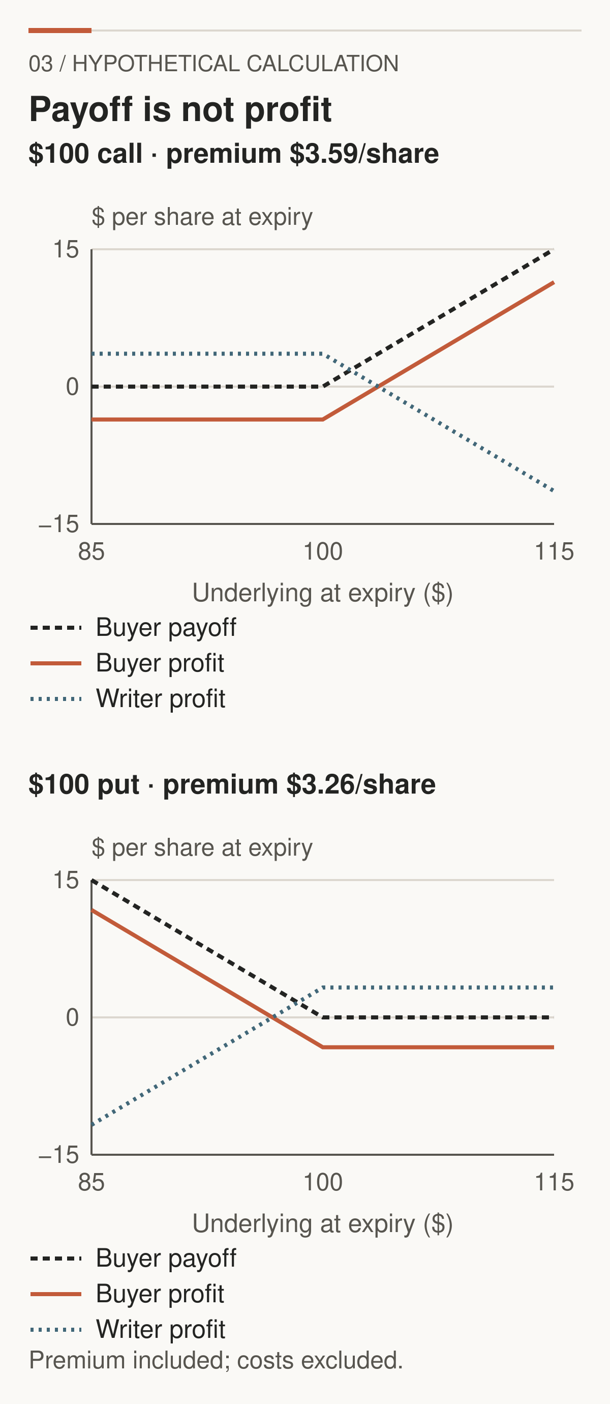
Figure 3. Hypothetical calculation. All curves describe expiry, not today's tradeable premium. Dashed charcoal is buyer payoff; solid terracotta is buyer profit; dotted blue is writer profit. Premiums are model outputs, with costs and financing excluded.
Before expiry, there is still a future. Intrinsic value is the positive exercise-price difference. Extrinsic value is the remaining premium beyond intrinsic value. It reflects more than a clock: uncertainty, rates, dividends, and exercise rights also matter. For some European options, discounting can even make premium less than the immediate-exercise intrinsic measure, so a universally positive “time-value bucket” is too simple.
Suppose the stock reaches $102 after one day, with 29 days left and unchanged volatility. Our call's model value becomes $4.6843: $2 intrinsic plus $2.6843 extrinsic. Selling at that model value would gain $109.32 per contract, even though stock remains below the expiry breakeven. The remaining option value explains the difference. An actual sale must use an available execution price.
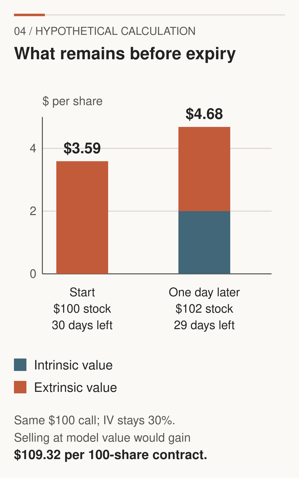
Figure 4. Hypothetical calculation. Expiry breakeven is not a barrier to taking a profit earlier. Black-Scholes inputs are stated in Section 3; only stock price and remaining time change here.
Exercise style and settlement are separate decisions in the contract design. American options permit exercise before expiry; European options permit it only at expiry. Cash settlement pays a specified cash difference. Deliverable settlement transfers an underlying position, which may be stock or futures. A long option's standalone loss limit is therefore different from the subsequent risk of a position created by exercise.
Pause and retain: strike determines contractual payoff. Premium and costs determine profit. Remaining time determines whether an expiry diagram describes the situation you are examining.
3. What a premium contains
Why does our call cost $3.59 rather than $1 or $8?
We use the Black-Scholes model for a European equity option with stock S = $100, strike K = $100, 30 calendar days remaining, annualised volatility σ = 30%, continuously compounded annual interest rate r = 4%, and dividend yield q = 0. Time is 30/365 years. The assumed multiplier is 100. The model treats volatility and rates as constant over the remaining life and uses a continuous diffusion for prices. Real markets can jump, have changing volatility, and charge execution costs. OIC: Black-Scholes inputs and limitations.
Change an input and the estimate changes. A higher stock price helps this call. A more distant strike makes the purchase right harder to use profitably. More uncertainty increases the value of this conventional optional payoff. Time permits more possible outcomes. Rates and dividends affect the economics of holding the asset versus holding an option. For commodities, carry and the futures price require a different formulation.
The model is an accounting language for these relationships, not a price-setting authority. It produces theoretical value. The last trade is a transaction that already happened, perhaps when stock or volatility was different. The mid-price is halfway between the current best bid and ask. It is a reference, not a guaranteed fill.
Suppose the hypothetical call has a bid of $3.50 and an ask of $3.68. Its midpoint is $3.59, close to our model value. An immediate small purchase may pay $3.68; an immediate sale may receive $3.50, subject to size and quote changes. A displayed last trade at $3.20 does not make $3.20 available. Nor does the midpoint erase the $18 contract-level spread between those quotes.
A ten-cent option is inexpensive in cash outlay, but it may be extremely unlikely to finish with value. “Cheap” requires a comparison between price and a defensible valuation, including the distribution of outcomes, costs, and your uncertainty about both. A low number on the screen is not that comparison.
The prices, sensitivities, and curves in this article come from the same inputs. The bid–ask examples are separately labelled invented execution scenarios. They are not independently invented Greeks attached to a convenient premium.
4. Pricing uncertainty
Volatility asks how much prices vary, not which direction they must travel.
Realised volatility is calculated from observed returns over a specified period. A common daily estimate takes the standard deviation of daily log returns and multiplies it by the square root of an assumed number of trading days in a year, often 252. The window, sampling frequency, estimator, and annualisation convention belong beside the number.
Implied volatility, or IV, works in the other direction. Given an option price and the model's other inputs, solve for the volatility that reproduces the price. It is a price translated into a model parameter. It contains the market's valuation of uncertainty, including risk compensation and supply and demand for options. It is not an objective forecast of future realised volatility. OIC: volatility concepts.
An approaching event can make a large jump more plausible. Buyers may pay more for optionality before the announcement. IV expansion describes rising implied volatility. IV crush describes a sharp fall, often after uncertainty is resolved. Neither requires the underlying to move much, and an event can leave substantial uncertainty behind.
Consider a separate event version of our $100 call: seven days left, stock and strike both $100, IV 60%, rate 4%, no dividend. It is worth $3.3511. One day later, stock is unchanged but IV falls to 30%, with six days remaining. It is worth $1.5670. The $178.41 contract loss comes from repricing the remaining opportunity, not from an adverse stock move.
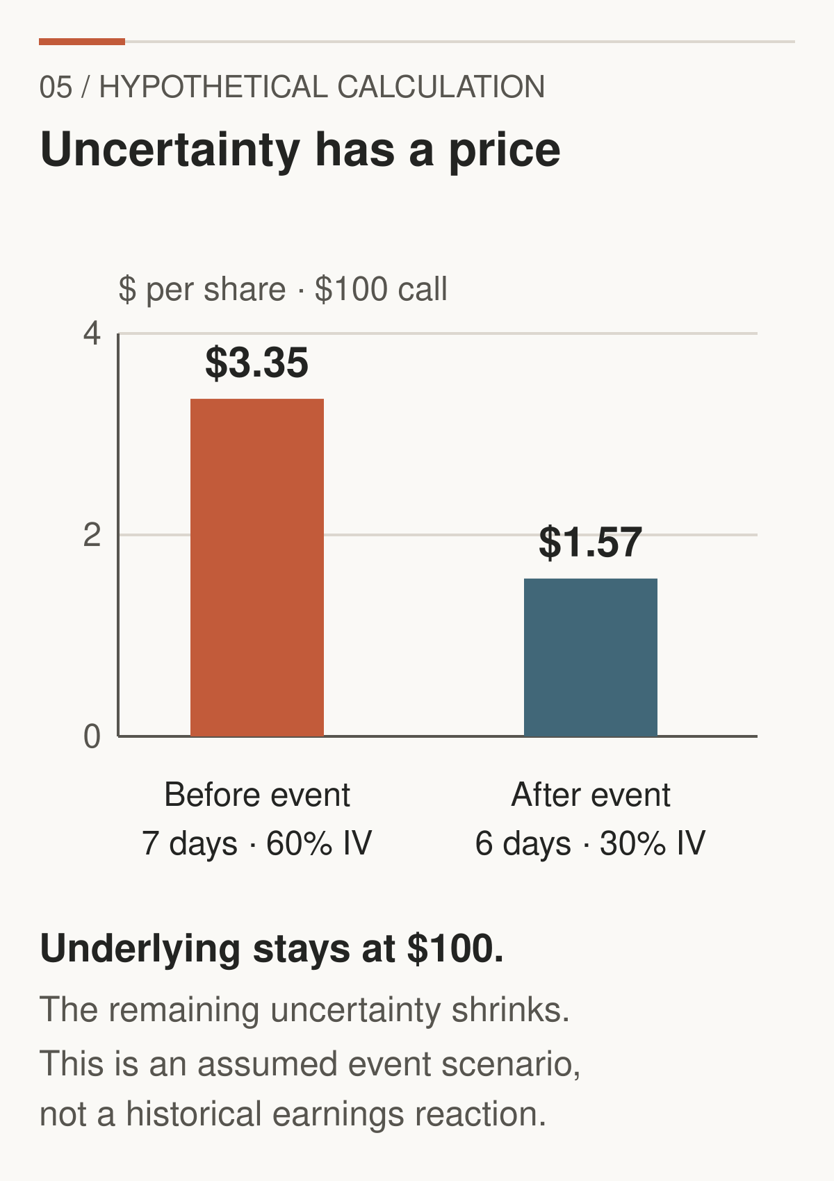
Figure 5. Hypothetical calculation. Both volatility and time change in this event scenario. The bars do not claim to isolate a pure volatility effect or describe an observed announcement.
IV also varies across strikes. A skew is a tilt in that relationship; a smile has relatively higher IV away from the middle. These shapes can reflect different tail risks and demand for protection. Across expiries, the volatility term structure compares IV for different horizons, ideally at a consistent moneyness or delta definition. A short expiry containing an event can have a higher annualised IV than a longer expiry. The longer option can still include more total variance, approximately σ²T.
That is different from a futures price curve, which compares prices for different delivery months. “Backwardation in oil” and “high near-term option IV” describe different objects. One cannot be substituted for the other.
A rough movement scale helps translate IV:
Movement scale ≈ underlying price × annualised IV × √(time in years).
Our inputs give $100 × 0.30 × √(30/365) = $8.60. This is a one-standard-deviation-style approximation, using a locally linear return approximation, square-root-of-time scaling, and a constant volatility assumption. It is not the expected absolute move. Under a centred normal approximation, expected absolute movement would instead be about 0.798 times that scale.
The frequently drawn $91.40–$108.60 band is therefore not a hard boundary, a price target, or a guaranteed 68% interval. Exact lognormal endpoints are asymmetric; jumps, skew, changing volatility, and the distinction between pricing and real-world probabilities weaken a literal probability reading. Do not combine an IV annualised under one convention with a time fraction from another without checking the conventions.
Two historical comparisons are often confused. IV rank conventionally places today's IV between the lookback minimum and maximum: 100 × (current − minimum)/(maximum − minimum). IV percentile conventionally reports the percentage of observations below today's IV. Definitions and tie handling can differ by provider. Specify, for example, 252 daily observations of the same 30-day at-the-money measure. A single extreme can distort rank; neither measure controls for a changed business or event regime. High IV is not automatically an option-selling opportunity: a large premium may compensate for a very large risk. Tastylive: rank and percentile conventions.
Volatility indices need the same specificity. Cboe's VIX concerns approximately 30-day S&P 500 option-implied volatility. CME's CVOL is a family of roughly 30-day measures derived from options on identified futures markets; its simple-variance methodology differs. Choose the relevant underlying before comparing them. A broad equity index is not the IV of a particular crude option. Cboe VIX fact sheet, CME CVOL methodology overview.
Pause and retain: IV describes how uncertainty is priced. It does not assign direction, certify fair value, or guarantee a future range.
5. Five questions answered by the Greeks
An option's premium depends on several moving inputs. The Greeks are local sensitivities: how much the model value changes when one input changes slightly and the others are held fixed. They are derivatives, not five independent forecasts.
Delta: what if the underlying moves?
Our call's delta is 0.53237. A small $1 stock rise contributes roughly $0.53237 per share, or $53.24 per assumed contract, before allowing for changing sensitivity. Ten long calls have approximately 10 × 100 × 0.53237 = 532.37 shares of delta. The put's delta is −0.46763, equivalent to −46.76 shares per contract.
Delta is a local price slope. It is not an exact real-world probability of profit. Even the probability of finishing in the money is different from recovering your premium. In this model, call delta uses N(d₁), while the model's risk-neutral expiry-in-the-money probability uses N(d₂). Neither supplies the real-world probability of a profitable exit at your chosen time. OIC: delta sensitivity.
Gamma: how quickly does delta change?
Our call and put both have gamma 0.04623 per $1 stock move. For a small $1 rise, call delta moves approximately from 0.53237 to 0.57860; put delta moves from −0.46763 to −0.42140. The put becomes less negative. That is positive gamma too.
Long conventional calls and long conventional puts have positive gamma in our model. Short positions reverse it. A contract name does not determine the sign of its owner's position gamma. Gamma itself changes with price, time, and volatility. OIC: gamma.
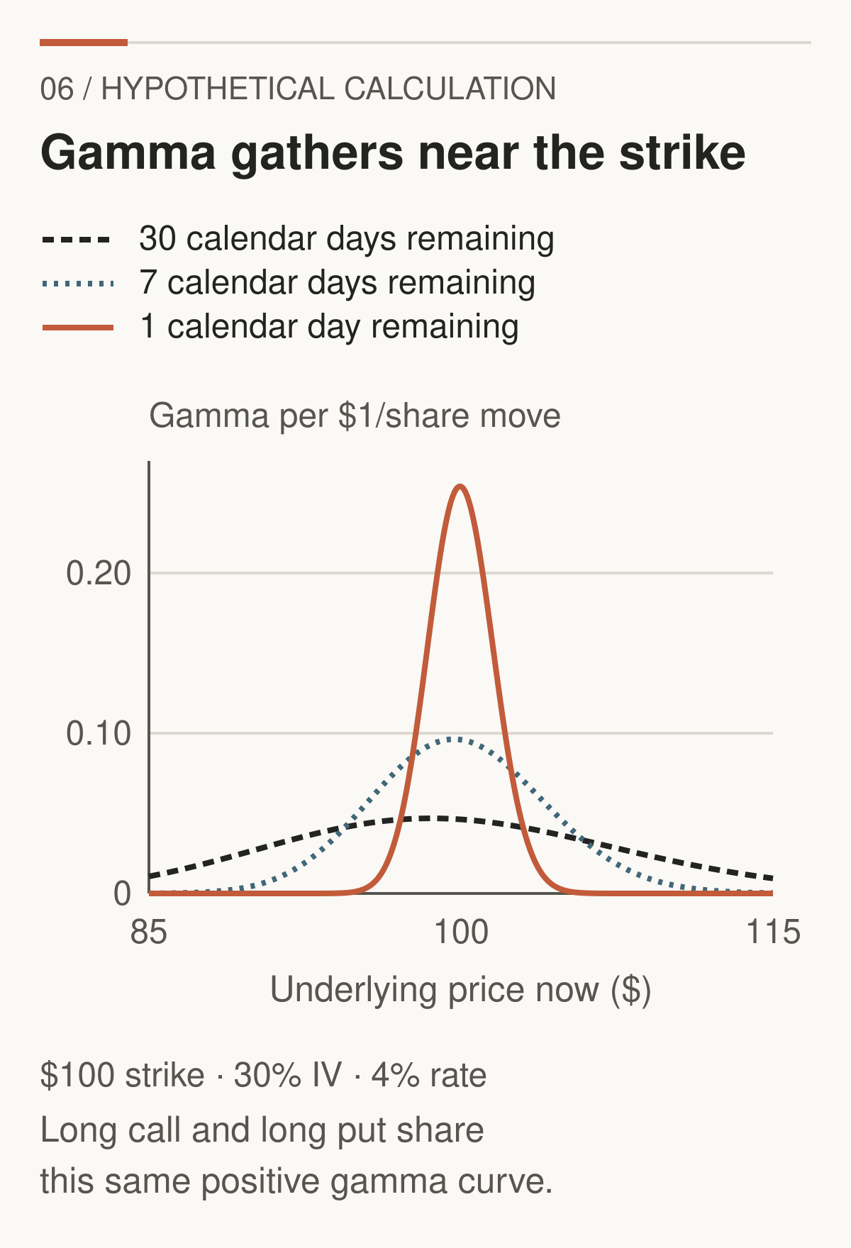
Figure 6. Hypothetical calculation. Black-Scholes gamma for the same $100 strike at 30, seven, and one calendar day remaining, with IV fixed at 30%. Near-expiry sensitivity concentrates around the strike; it is not enormous for every expiring option.
Theta: what if time passes?
Our call's theta is −$0.06244 per share per elapsed calendar day. Its local one-day contribution is about −$6.24 per contract. Full repricing after one day, with other inputs fixed, gives a $6.29 decline. The small difference appears because theta changes too.
Time decay is not a fixed daily fee. Its shape depends on moneyness, volatility, rates, dividends, and exercise rights. The negative sign applies to our example; some long European puts can have positive theta in other circumstances. A model's calendar-day convention also need not match how the market prices a weekend or a specific event. OIC: theta.
Vega: what if implied volatility changes?
Our call's vega is $0.11400 per share per percentage point of IV. A move from 30% to 31% contributes about $11.40 per contract. A 1% relative increase from 30% is only 30.3%, so its local contribution is about $3.42 per contract. The two changes are different sizes.
Long calls and puts have positive vega here. Vega is not constant across strikes, maturities, or large volatility moves. A single number also cannot describe every change in a whole volatility surface. OIC: vega.
Rho: what if rates change?
Our call's rho is +$0.04080 per share per percentage-point increase in the annual interest rate. Moving r from 4% to 5% contributes about $4.08 per contract locally. The matching put's rho is −$0.04112 per share per point. These signs describe this equity pricing formulation with spot and dividends fixed. They must not be transferred blindly to futures options, where holding the futures price fixed changes the calculation. OIC: rho.
| Sensitivity | Long call | Long put | Short call | Short put |
|---|---|---|---|---|
| Delta | Positive | Negative | Negative | Positive |
| Gamma | Positive | Positive | Negative | Negative |
| Theta, at our inputs | Negative | Negative | Positive | Positive |
| Vega | Positive | Positive | Negative | Negative |
| Rho, spot held fixed | Positive | Negative | Negative | Positive |
This reference describes vanilla European equity options under our assumptions. For a portfolio, multiply each per-share Greek by the signed number of contracts and 100, then sum. Net sensitivities can hide offsetting positions with very different behaviour under a larger shock.
Putting the inputs back together
Now let stock rise from $100 to $101, five calendar days pass, and IV fall from 30% to 20%. Keep the strike, rate, and dividend assumption unchanged. Using initial Greeks, the local approximation is:
ΔV ≈ delta × ΔS + ½ gamma × (ΔS)² + theta × elapsed days + vega × ΔIV in percentage points + rho × Δr in percentage points.
The per-share contributions are +$0.53237 from delta, +$0.02312 from gamma, −$0.31219 from theta, and −$1.13996 from vega. Rates contribute zero. The total is approximately −$0.89667.
Full model repricing gives a new premium of $2.79357, a decline of $0.79755, or $79.75 per contract. The approximation misses by $0.09912 per share. Five days and a ten-point IV drop are substantial changes; omitted cross effects and higher-order terms matter.
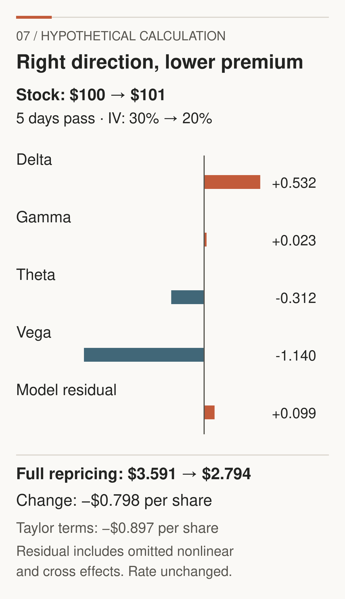
Figure 7. Hypothetical calculation. The bar contributions are local Taylor terms, not uniquely identifiable realised causes. Adding the +$0.09912 model residual reconciles them with full repricing. The underlying rises, but the option loses value.
Optional advanced note: vanna measures how delta changes with volatility, under a stated volatility unit; charm measures how delta changes with time, whose sign depends on whether time means elapsed time or time remaining. Either can change hedge needs without a stock move. The direction depends on the signed portfolio and the convention. “IV falls, so dealers must buy” is incomplete without those details.
Pause and retain: the Greeks explain why direction can be right while the option loses. They describe sensitivities now; they do not promise tomorrow's execution price.
6. From an option to a hedge
How can an options trade generate buying or selling in the underlying?
A market maker quotes prices and accepts inventory risk while facilitating transactions. A customer may trade with a dealer, another customer, or through arrangements that involve several participants. Clearing organises contractual obligations and counterparty risk; it does not mean the clearing house takes the directional market view suggested by the trade.
Suppose a dealer is short ten calls, each representing 100 shares, with delta 0.50. These rounded deltas are a separate hedge-arithmetic illustration, not our exact Black-Scholes outputs. The option position has −10 × 100 × 0.50 = −500 shares of delta. Buying 500 shares would approximately offset that sensitivity.
If stock rises and the call delta becomes 0.60, the option position now has −600 shares of delta. A dealer choosing to restore neutrality buys another 100 shares. On a decline that reduces delta to 0.40, the desired hedge becomes 400 shares, requiring a sale of 100. This short-option book trades with the price move in the fixed-book example.
A dealer long the same calls starts with +500 shares of delta and could short 500 shares. If delta rises to 0.60, the dealer shorts another 100 shares. If delta falls to 0.40, the dealer buys back 100. Positive-gamma rebalancing trades against the price move. The arithmetic follows directly from delta and gamma, not from a dealer's presumed forecast. CME: gamma and changing delta.
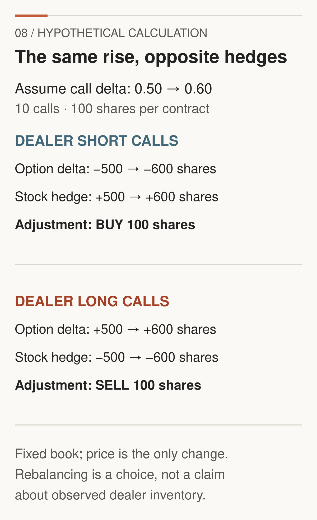
Figure 8. Hypothetical calculation. Option sensitivity changes, then a dealer choosing to rebalance adjusts the underlying hedge. Inventory, time, and volatility are otherwise fixed. Actual dealer positions and transactions are not observed.
Check the put rather than memorising a call-only story. Ten long puts at delta −0.50 have −500 shares of delta and could be hedged by buying 500 shares. After a stock rise makes put delta −0.40, only 400 hedge shares are needed: sell 100. A dealer short those puts has the opposite position and buys 100 shares to reduce the initial short-stock hedge. Again, long-option gamma is positive; short-option gamma is negative.
Dealers manage portfolios, however. Calls, puts, futures, shares, and other hedges can net against one another. New trades, volatility changes, time passing, risk limits, transaction costs, and liquidity all change the desired adjustment. A dealer may hedge in a correlated instrument or rebalance intermittently. The local hedge calculation is therefore a potential mechanism, not a record of an order that must occur.
Delta-neutral is not risk-free. Gamma, volatility, jumps, imperfect hedges, financing, and execution remain. A neutral snapshot can become directional a moment later.
7. What GEX measures, and what it assumes
Gamma exposure, usually shortened to GEX, extends that hedge calculation to a collection of options. Before reading a colourful strike map, identify which of four different things it contains.
One option's gamma is a sensitivity. Unsigned open-interest-weighted gamma weights its magnitude by outstanding contracts. A signed dealer scenario additionally assumes how many contracts dealers hold long or short. Observed dealer inventory requires actual position information. An ordinary aggregate chain does not provide that final ingredient.
Open interest, or OI, counts outstanding contracts. Every contract has a long and a short. There is no market-wide surplus of option longs over shorts to discover by counting calls. OI does not say which side belongs to a dealer, or reveal offsets outside the chain. CFTC: open interest and report construction.
Our default dealer-positioning label is therefore UNKNOWN. Signing every call positive and every put negative is an inventory assumption if a model uses it. It is never an inherent property of calls and puts.
Deriving a convention instead of memorising a formula
Let n be signed option contracts, positive for long and negative for short; M the shares per contract; Γ the per-share gamma; and S the positive stock price.
The position's share delta is n × M × delta. For a small stock change ΔS, its share-delta change is approximately n × M × Γ × ΔS. A 1% price rise substitutes ΔS = 0.01S. Multiply the resulting shares by S to express their current dollar notional:
GEX per 1% move ≈ n × M × Γ × S² × 0.01.
For our one long call, 1 × 100 × 0.0462319 × 100² × 0.01 = +$462.32 per 1% move. The option's delta increases by about 4.623 shares. Restoring a delta-neutral hedge would require selling those shares, the opposite sign to the option-delta change.
This definition is a dollar hedge-notional sensitivity, not a cash profit. Dollar hedge-notional sensitivity per $1 underlying move is instead nMΓS. Gamma's local contribution to option profit is ½nMΓ(ΔS)². At S = $100, a 1% move happens to equal $1, making the first two numbers coincide; that accident disappears at other prices.
A chain whose assumptions can be inspected
Here is the entire hypothetical chain, pairing a call and put at each strike and expiry. All use S = $100, IV 30%, r = 4%, q = 0, European exercise, ACT/365, and M = 100.
| Days left | Strike | Call OI | Put OI |
|---|---|---|---|
| 7 | $90 | 200 | 1,200 |
| 7 | $100 | 1,500 | 1,500 |
| 7 | $110 | 1,200 | 200 |
| 30 | $90 | 400 | 800 |
| 30 | $100 | 1,000 | 1,000 |
| 30 | $110 | 800 | 400 |
Unsigned exposure is $4.523 million per 1% move, counting each contract once, not adding both its long and short sides. It describes a scale of sensitivity, not net dealer exposure.
We calculate three independent inventory scenarios. A assumes dealers are net short 25% of each series' OI. B assumes dealers are net long 25% at $90, flat at $100, and net short 25% at $110, for both calls and puts. C reverses B. The remainder is outside the assumed net dealer book. None of these fractions is measured.
At $100, A produces −$1.131 million, B −$37,086, and C +$37,086, all per 1% move. Identical public OI supports all three constructed results because the missing inventory assumptions differ.
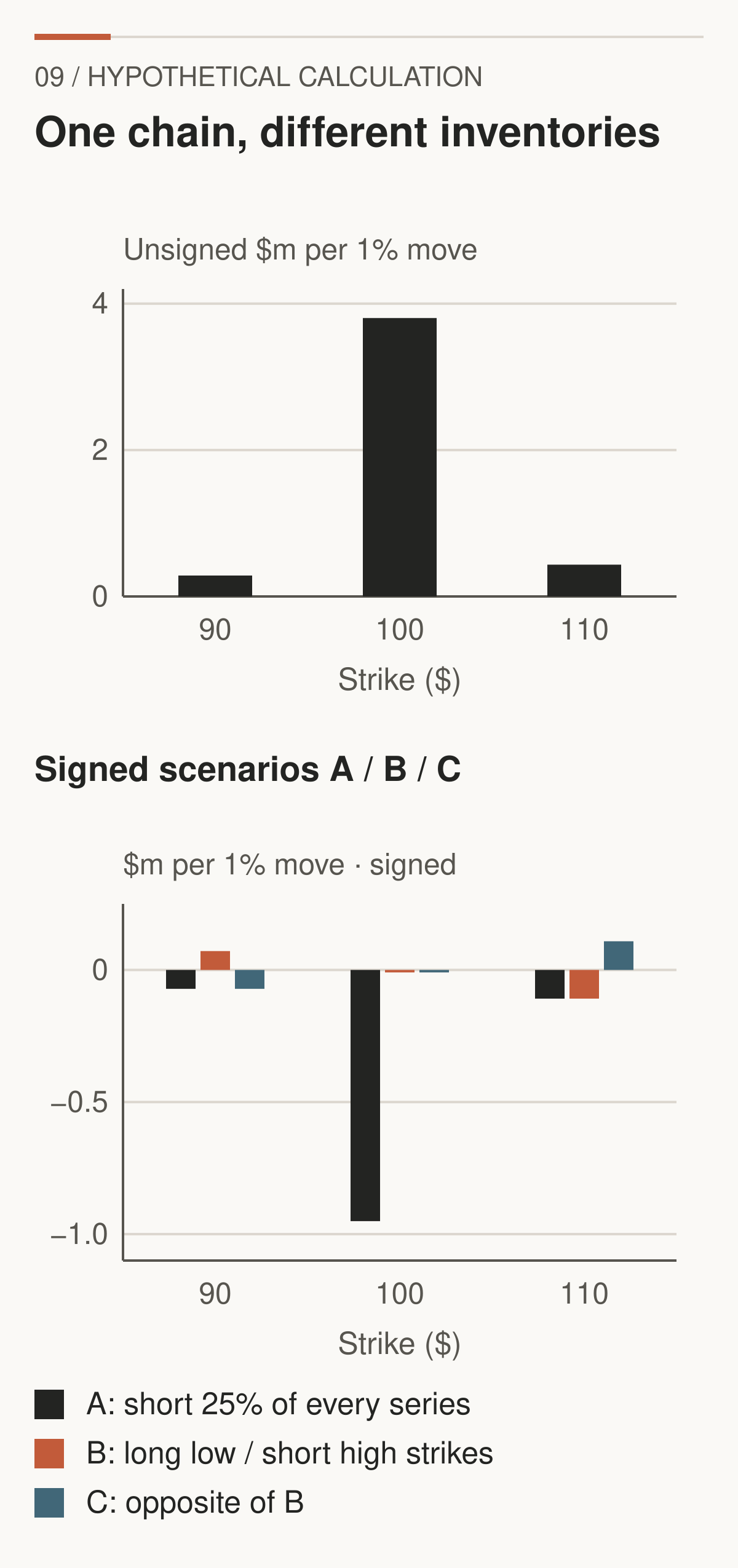
Figure 9. Hypothetical calculation. Upper panel: unsigned magnitude. Lower panel: signed scenarios at S = $100, aggregated across both expiries, with A, B, and C ordered left to right at each strike. Call and put gamma are both positive before position signs are applied. Units are millions of dollars of hedge-notional sensitivity per 1% move.
Expiry aggregation matters too:
| Days left | Unsigned | Scenario A | Scenario B |
|---|---|---|---|
| 7 | $3,033,131 | −$758,283 | −$14,248 |
| 30 | $1,490,312 | −$372,578 | −$22,838 |
| Total | $4,523,443 | −$1,130,861 | −$37,086 |
Scenario C reverses B. Small rounding differences may occur when adding displayed amounts. These are sensitivities at one instant, not scheduled future orders.
A zero-gamma level, sometimes called a gamma flip, is a trial underlying price at which a chosen signed exposure model crosses zero. To find it, we recompute each option's gamma at every trial price. Accumulating today's strike bars answers a different question and cannot substitute for repricing.
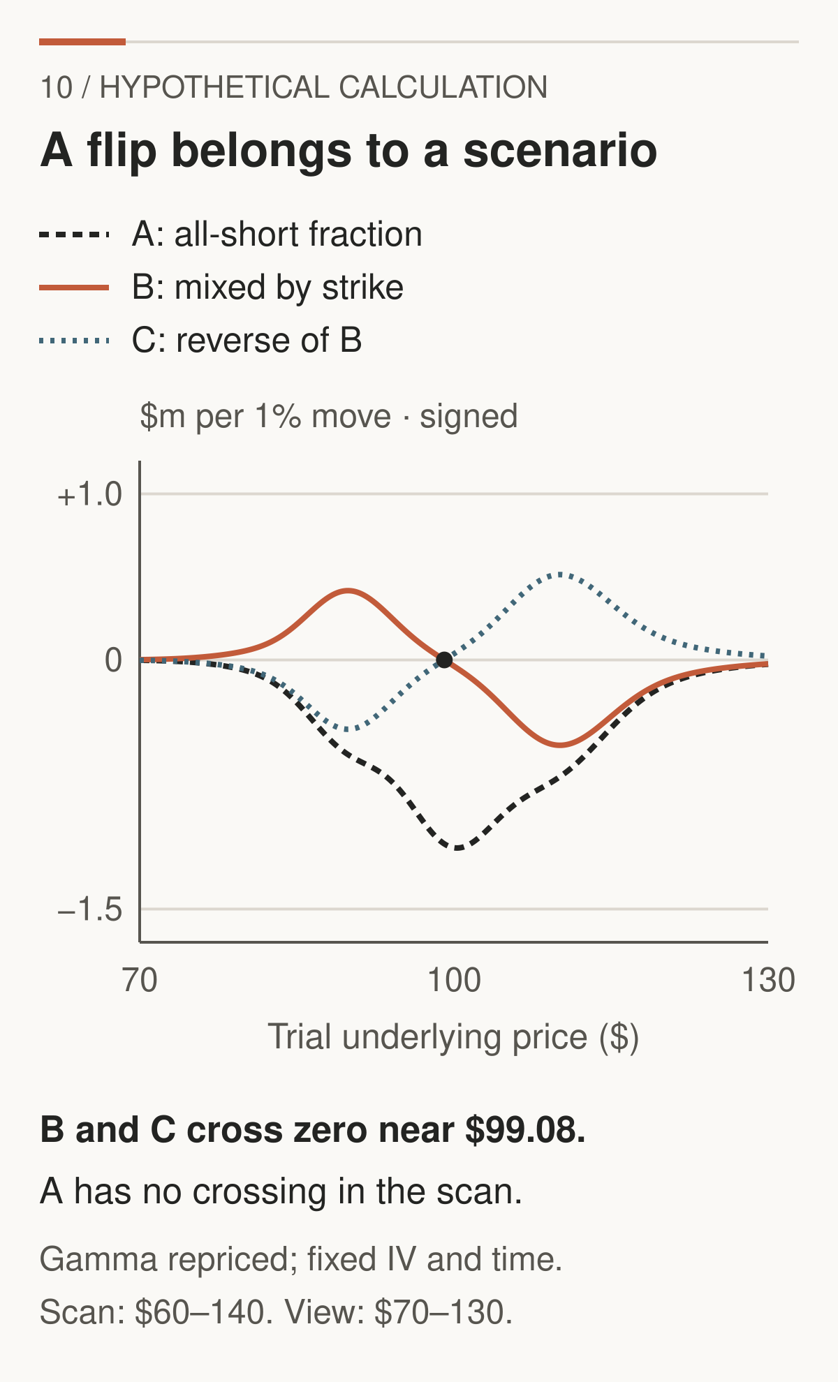
Figure 10. Hypothetical calculation. The scan runs from $60 to $140 in $0.10 steps, followed by root refinement; the chart displays $70–$130. Time, inventory, rates, and 30% IV at every strike are fixed. B and C cross near $99.08. A has no crossing anywhere in the scan and is negative for every positive price under this all-short model.
The flat, fixed-IV surface is deliberately simple. A different surface response, signed book, or time snapshot can move or remove a crossing; a more complicated book can have several. No crossing is a valid result. The $99.08 here is an answer to an invented calculation, not a level in any traded market.
A gamma concentration identifies where sensitivity is large under the chosen weighting. Vendor “call walls” and “put walls” may refer to different OI or exposure measures; read the definition. Pinning is an interpretation that hedging or other activity contributes to trading near a strike around expiry. Large OI alone does not establish a magnet, support, resistance, or causation.
Finally, translate scale into liquidity. Scenario A's local sensitivity at $100 corresponds to about 11,309 shares of potential hedge adjustment for a 1% rise. If an invented comparison market trades 500,000 shares during the relevant interval, that is about 2.3% of interval volume. It still says nothing definite about impact: execution speed, replenishment, cancellations, other flows, and the decision to hedge matter. Daily notional and instantaneous order-book depth are different denominators.
Pause and retain: GEX is useful conditional arithmetic. An inventory assumption does not become observed positioning because the chart is precise.
8. Reading an options tape
What actually happened when an options trade printed?
Volume counts contracts traded during an interval, rather than the number of separate prints. Open interest counts contracts remaining outstanding at a snapshot. A buy can open a long position or close a short; a sell can open a short or close a long. The paired counterparties determine the OI change. CME: volume and open interest.
| Buyer action | Seller action | One traded contract changes OI by |
|---|---|---|
| Buy to open | Sell to open | +1 |
| Buy to close | Sell to close | −1 |
| Buy to open | Sell to close | 0 |
| Buy to close | Sell to open | 0 |
Start with OI of 100. Ten contracts opened on both sides raise OI to 110. If those same ten later close against one another, OI returns to 100, while the two transactions contribute 20 to volume. Repeat that sequence and volume can exceed yesterday's OI without a large change in final inventory. Volume above previous OI does not prove every trade opened a position.
Public trade records can report time, series, quantity, price, venue, and trade conditions. A quote feed can supply contemporaneous bids and asks. Aggressor classification then estimates who demanded immediate execution. A print at the ask is often classified as buyer-initiated; one at the bid as seller-initiated. A midpoint print is less informative. Stale quotes, mismatched clocks, delayed reports, price improvement, and complex executions can defeat the simple rule. Cboe's trade-data documentation illustrates the observed fields and separately calculated analytics. Cboe Option Trades.
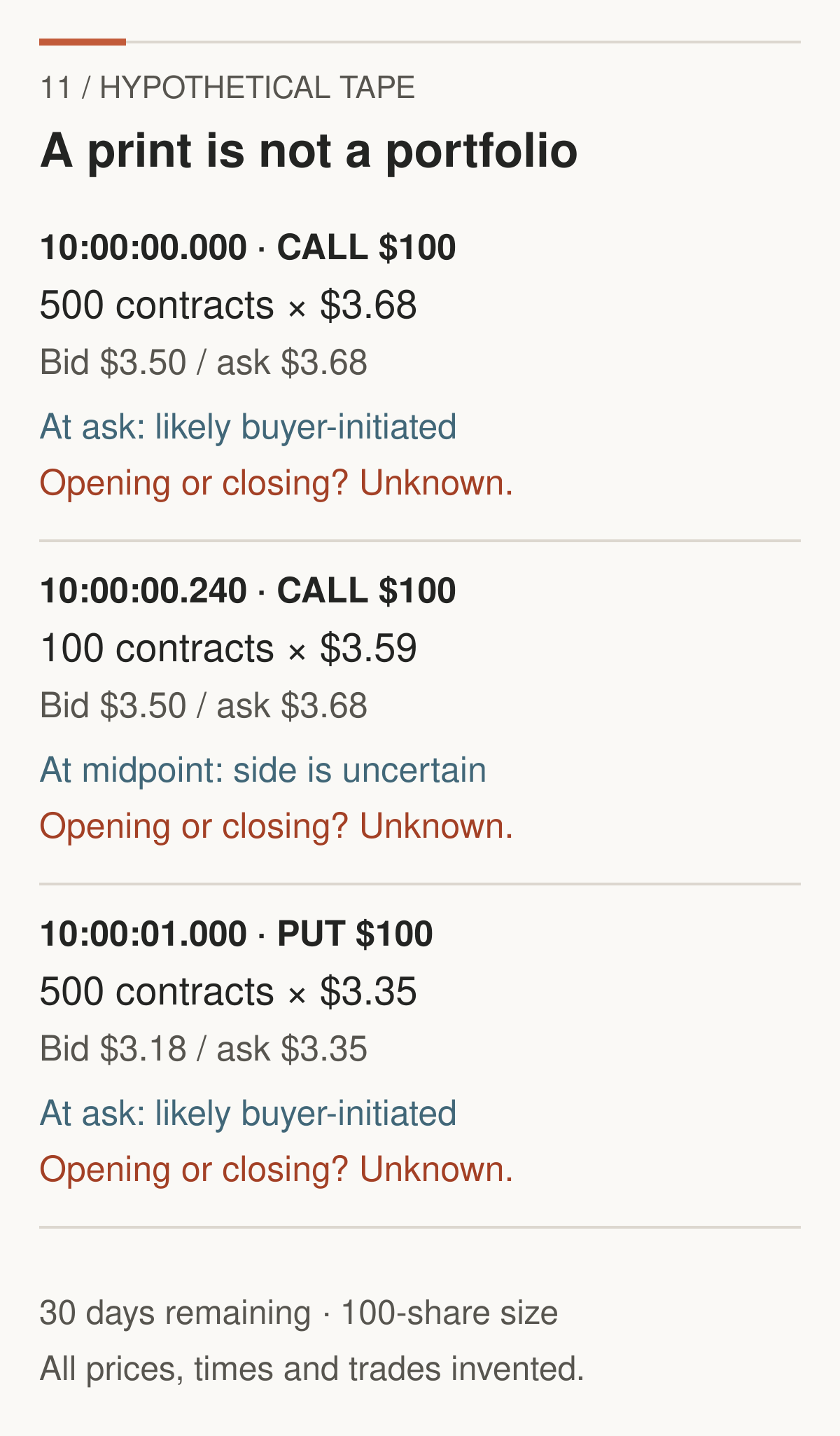
Figure 11. Hypothetical tape. All timestamps, quotes, sizes, and prints are invented. “Likely buyer-initiated” is an inference from the assumed aligned quote, not an exchange open/close flag. The example uses 30-day $100 options and the assumed 100-share multiplier.
Our first call print is 500 contracts at $3.68, with a $3.50 bid and $3.68 ask. Reported gross premium is $184,000. If the buyer is newly long, the option leg adds approximately 26,619 shares of delta, using our initial model delta. If it closes 500 short calls, it instead removes the negative delta of that short position. In either case, the buyer's option-position delta increases locally, but the portfolio and purpose can be completely different.
The purchase might be outright speculation, protection for short shares, one leg of a vertical spread, or short covering. A nearby transaction at another strike might suggest a spread, but proximity alone does not prove a linkage. The put purchase in the tape may protect a much larger long-stock portfolio, leaving its owner net bullish. Premium paid is not the same as net risk, delta exposure, capital committed to the whole strategy, or conviction.
Multi-leg orders trade combinations. Rolls close an existing exposure and open another, often at a later expiry. Blocks follow exchange-specific rules for large negotiated trades. Sweeps, in many retail feeds, group executions across available liquidity or venues. None of these labels alone establishes informed, opening, directional demand. A vendor's grouped “sweep” can also be an inference rather than a directly reported exchange instruction.
Some exchange datasets do explicitly distinguish participant capacity, buy/sell, and open/close. Cboe's dedicated Open-Close product is an example, with stated exchange coverage. Those fields are different from a vendor inferring intent from price. Even genuine flags do not reveal the participant's entire cross-market portfolio. Cboe Open-Close documentation.
Interpretation improves when aligned quotes, price response, IV changes, reliable flags, and subsequent OI point in a compatible direction. It remains an interpretation. Next-day OI is an aggregate net result affected by other trades, exercises, and expiry; it cannot generally identify the opening status of one print.
The same restraint applies to put/call ratios and “unusual activity”. State whether a ratio uses volume or OI, which expiries it includes, and whether large trades or rolls dominate it. A departure from an average describes unusual measured activity. It does not supply a trading instruction.
9. The auction underneath the options
An option hedge eventually meets someone else's order.
A bid offers to buy; an offer, or ask, offers to sell. Their difference is the spread. A marketable order accepts available prices, while a passive limit order waits. Depth is the quantity available across prices. Quotes can be cancelled or revised, so a displayed book is a temporary opportunity, not a commitment to absorb unlimited trading.
Suppose sellers offer 100 shares at $100.00 and 100 at $100.02. A marketable purchase of 150 shares, against that fixed book, fills 100 at $100.00 and 50 at $100.02. Its average is about $100.0067. The final execution is higher because the first price had insufficient quantity. Real books can change during this process.
Every execution still has a buyer and seller. Buying pressure concerns aggressiveness and available liquidity, not a greater count of buyers. Price impact depends on the orders encountered and the information inferred, as well as on quantity. This is why a hedge-notional estimate cannot simply be converted into a guaranteed price change.
Absorption describes a possible pattern in which aggressive executions repeatedly meet replenishing passive liquidity with limited price progress. Establishing it requires suitable execution and quote data, accurate side classification, and a chosen interval. A candle alone does not reveal the sequence or identify the resting participant.
Options delta is a price sensitivity. Order-flow delta is commonly buy-initiated volume minus sell-initiated volume, under a feed's classification. Cumulative volume delta adds those imbalances over an interval. Products that estimate aggressors from candle direction are different from feeds with trade-level information. Similar terminology does not make the measurements interchangeable.
Stops can turn into marketable orders after a trigger, depending on order type. They do not guarantee a fill at that trigger. Short covering creates purchases to reduce short exposure; it need not express a fresh bullish belief. Leverage-driven liquidation follows a financing or risk constraint. Funding trouble can reduce both the ability to hold positions and the willingness to supply liquidity, reinforcing a move under some conditions. Brunnermeier and Pedersen: market and funding liquidity.
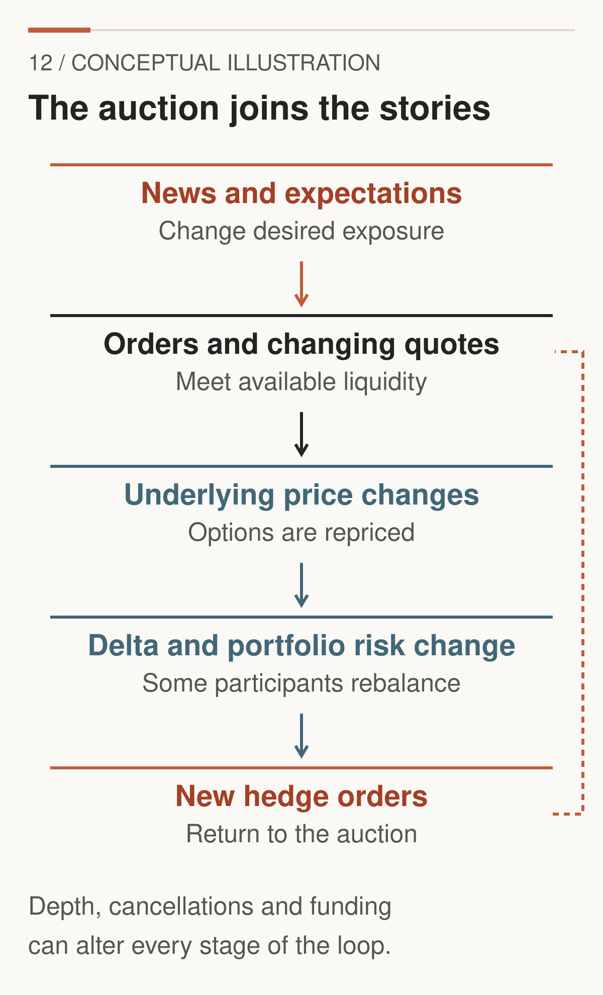
Figure 12. Conceptual illustration. Options hedging is one feedback channel inside a wider auction. News, liquidity, funding, and other portfolio decisions can initiate, reinforce, or overwhelm it. This is a mechanism map, not evidence of a particular market's cause.
| Evidence | Useful for | Cannot establish alone |
|---|---|---|
| Price action | Where prices moved and whether a move persisted | Participant identity or motive |
| VWAP | Comparison with a volume-weighted price over a defined session or anchor | Fair value or guaranteed support |
| Volume | Amount traded over a defined interval | Net bullish conviction |
| Open interest | Outstanding contract count and its change | Which side dealers own |
| Options flow | Observed transactions and qualified aggressor estimates | Whole portfolios or unknown opening intent |
| GEX estimates | Sensitivity under an explicit signed-inventory model | Certain hedge trades or causal market impact |
| CFTC positioning | Delayed aggregate exposures by reporting category | An intraday trigger or a dealer gamma map |
The CFTC's futures-and-options-combined reports use delta-adjusted futures equivalents. They are not gamma exposures. Their categories and reporting dates belong alongside any positioning conclusion. CFTC explanatory notes.
Four conditional scenarios bring these distinctions together:
A positive-gamma range. Assume a sufficiently large net long-gamma intermediary book and repeated rebalancing. Selling rises and buying falls could add opposing flow. Range trading alongside independently supported inventory estimates would be compatible evidence. Persistent directional news, small hedge size, or evidence that the book is short gamma weakens the interpretation. The range itself does not establish the inventory.
Negative-gamma amplification. Assume net short gamma, active rebalancing, and limited liquidity. A rise raises option delta and may prompt purchases; a fall may prompt sales. Accelerating moves accompanied by aligned hedge-flow evidence fit the mechanism. Deep replenishing liquidity, large opposing flows, or absent rebalancing weakens it. Momentum alone is insufficient.
An event followed by IV crush. Assume a known uncertainty is resolved and remaining implied volatility falls. An option can lose despite a favourable underlying move, as our repricing showed. Compare the same contract, time, and executable quotes. A stale last trade, widened spread, or changing strike comparison can undermine the claimed explanation.
Expiry or a roll changes exposure. Assume contracts expire or positions move into different maturities. Their gamma weights can disappear, concentrate, or migrate, changing the estimated book. Expiry-level OI, identified roll legs, and fresh calculations are relevant observations. Offsetting new positions or unverifiable opening flags weaken a simple “hedges must unwind” narrative. Exercise can also create underlying exposure rather than simply eliminate risk.
These are teaching scenarios, not recommendations. Fundamentals change desired exposures; news is evaluated against expectations; liquidity determines execution; hedging and funding can alter the path. Options are part of that explanation, not a universal substitute for it.
10. Taking the framework to WTI and MCX
“Crude oil options” is not a sufficiently precise instrument name.
Identify the exchange, product, exact underlying futures month, option expiry, strike, multiplier, quotation currency, and settlement rules. An option expiring this month may reference a futures contract with a different named delivery month. A continuous chart is not itself the hedgeable contract.
The exchange documents available on 19 September 2026 distinguish the following standard products:
| Feature | NYMEX standard WTI option | MCX standard CRUDEOIL option |
|---|---|---|
| Underlying | Specified CL futures contract | Specified MCX crude futures contract |
| Contract exposure | One 1,000-barrel CL future | One 100-barrel MCX crude future |
| Premium quotation | US dollars per barrel | Indian rupees per barrel |
| Exercise style | American under Chapter 310 | European under March 2026-onwards specification |
| Option expiry rule | Third business day before underlying futures expiry | Two business days before underlying futures expiry |
| Exercise consequence | Underlying futures position | Devolvement into underlying futures position |
Sources: NYMEX option Rule 310, NYMEX futures Rule 200, and MCX March 2026-onwards option specification. The table does not cover every weekly, mini, micro, or other crude product.
NYMEX CL futures have physical-delivery rules. The current MCX standard crude futures specification instead links final settlement to the NYMEX CL front-month settlement converted using the specified RBI USD/INR reference rate. The MCX future is cash-settled, but option exercise can first create that futures position and its associated margin exposure. MCX futures specification.
MCX's option document describes automatic exercise of in-the-money options unless valid contrary instructions apply, and assignment to short positions. Devolved futures are opened at the option strike. Long calls and short puts become long futures; long puts and short calls become short futures. Funding, pre-expiry margins, broker cutoffs, and risk controls must therefore be checked for the actual contract and account, not inferred from the original premium debit.
Converting delta without importing the stock multiplier
If an option's premium is quoted per barrel and its delta is the premium change per one-unit change in its matching futures price F, then n options with multiplier Mₒ have monetary sensitivity n × Mₒ × delta per price unit. One hedge future with multiplier M𝒇 has sensitivity M𝒇. The matching futures equivalent is therefore n × Mₒ × delta / M𝒇.
When option and future multipliers match, ten options at delta 0.50 correspond to five futures, not 500 futures. For standard WTI, that is $5,000 sensitivity per $1/barrel move. For standard MCX crude, it is ₹500 per ₹1/barrel move. The 100-share example is irrelevant to these dimensional conversions.
For a European futures-option illustration, Black-76 discounts an optional payoff on the futures price. With F = K = $80/barrel, 30/365 years, IV 35%, and rate 4%, it gives a call premium of $3.1906/barrel, delta 0.51830, and gamma 0.049472 per $1/barrel move. With 1,000 barrels, premium is $3,190.60. This is a European model illustration, not a claim that NYMEX's American exercise feature disappears. MCX's published specification uses Black-76 for specified base-price and price-band calculations; market prices and operational rules remain distinct.
Define futures GEX explicitly as n × Mₒ × gamma_F × F² × 0.01, where gamma_F differentiates premium delta with respect to the futures price. For one long illustrative WTI-sized option it is about +$3,166.24 per 1% futures move. A hedge adjustment has the opposite sign. Holding F fixed in Black-76, rho is −T times option value per unit rate change, so both long calls and puts have negative rate sensitivity under that convention. This is why the equity sign table cannot simply travel to futures.
MCX trading can influence local futures through hedging and the local auction. International benchmarks, the rupee exchange rate, basis differences, trading hours, and liquidity connect that auction to other markets. Local option OI neither mechanically sets global crude prices nor becomes irrelevant merely because the benchmark is international.
Finally, a chart switching between futures months can jump because the two contracts have different prices. Back-adjustment changes historical levels too. Match the chart month to the option's actual underlying before calling such a discontinuity a rally, crash, breakout, or hedge trigger.
The companion essay, Why Bullish Oil Markets Still Pull Back, explores the wider distinction between a market thesis and the path prices take. Options add another layer of conditional exposure to that same auction.
Interpretation checklist
Before turning an options chart into a market story, ask:
- Which contract and clock? Underlying, month, expiry, multiplier, exercise and settlement.
- Which price? Trade, quote, midpoint, or model value, with a timestamp and available size.
- Which units? Per share or barrel, per contract, per day, per volatility point, or per 1% move.
- Which position? Long or short, standalone leg or portfolio; observed inventory or assumed fraction of OI.
- Which model? Pricing method, volatility surface, time convention, and repricing assumptions.
- Which evidence? Transaction facts, inferred aggressors, genuine flags, or unknown motives.
- Which competing explanation? News, liquidity, funding, rolls, and offsetting flows.
- What would weaken the story? Name an observation that could contradict it.
The payoff defines the contract. Pricing inputs value its remaining possibilities. Greeks describe local changes. Hedging can turn those changes into orders. GEX estimates the sensitivity of an assumed book. Flow reveals transactions with varying amounts of context. Underlying liquidity determines how orders can execute.
Keeping those links separate does not remove uncertainty. It makes the uncertainty visible, which is a better foundation for understanding than a confident label on an incomplete chart.
Educational note: This article explains mechanisms and hypothetical calculations, not personalised investment advice or trade recommendations. Options and futures can create substantial losses and obligations. Verify the current exchange and broker rules for any actual position.
Six questions to carry away
1. Can an in-the-money option lose money? Yes. Our call pays $2 at expiry after costing $3.5911. Being ITM describes payoff relative to strike, not profit after premium and costs.
2. Can a call lose value while the underlying rises? Yes. In our combined example, stock rises $1, but five elapsed days and a ten-percentage-point IV fall reduce model value from $3.5911 to $2.7936. Direction is only one input.
3. Can a long put have positive gamma? Yes. As stock rises, its negative delta becomes less negative. That is an increase in delta, hence positive gamma. Shorting the put reverses the position's gamma.
4. Does large call volume identify bullish customer positioning? No. Volume alone does not identify the aggressor, customer, opening status, other legs, or whole portfolio. A call purchase can close a short or hedge another exposure.
5. Can OI establish dealer gamma? No. It counts contracts with both a long and a short. Assigning a dealer side requires additional data or an explicitly labelled assumption. Reversing our assumed inventory reverses GEX.
6. Why might expiry change a GEX estimate? Remaining time changes gamma, especially near the strike; expired series disappear, positions may roll, and exercise may create underlying exposure. A fresh estimate must update both contract state and inventory assumptions.
Essential glossary
| Term | Meaning in this article |
|---|---|
| Underlying | Asset or futures contract referenced by the option |
| Premium | Price paid or received for the option |
| Strike / expiry | Contractual exercise price / end date |
| Multiplier | Converts quoted per-unit amounts into a contract amount |
| Exercise / assignment | Use of the right / allocation of the writer's obligation |
| Intrinsic / extrinsic | Exercise-price difference / remaining premium beyond it |
| IV / realised volatility | Volatility implied by an option price / measured from past returns |
| Moneyness | Relationship between underlying price and strike |
| Delta / gamma | Premium sensitivity to price / delta sensitivity to price |
| Theta / vega / rho | Sensitivities to elapsed time / IV / rates, with explicit units |
| Delta hedge | Offset to local directional sensitivity |
| Open interest / volume | Outstanding contracts / contracts transacted during an interval |
| GEX | A specified gamma-exposure convention, often conditional on inventory assumptions |
| Aggressor | Side seeking immediate execution against available liquidity |
| Basis | Difference between related prices or instruments |
| Roll | Closing one contract exposure and opening another |
Optional technical appendix
Pricing and Greek conventions
Let T be remaining calendar days/365; σ, r and q are annual decimal inputs. N is the standard normal cumulative distribution function and φ its density.
d₁ = [ln(S/K) + (r − q + σ²/2)T] / (σ√T)
d₂ = d₁ − σ√T
Call = S exp(−qT)N(d₁) − K exp(−rT)N(d₂)
Put = K exp(−rT)N(−d₂) − S exp(−qT)N(−d₁)
Gamma for either long option is exp(−qT)φ(d₁)/(Sσ√T). Vega per one percentage point is S exp(−qT)φ(d₁)√T/100. Theta is the negative derivative with respect to remaining time, divided by 365; rho is the derivative with respect to the decimal rate, divided by 100. The included code gives the complete formulas and validates them against finite differences and put–call parity.
| Quantity, per share | $100 call | $100 put |
|---|---|---|
| Premium | 3.591123 | 3.262896 |
| Delta | 0.532370 | −0.467630 |
| Gamma, per $1 move | 0.046232 | 0.046232 |
| Theta, per elapsed day | −0.062439 | −0.051516 |
| Vega, per IV percentage point | 0.113996 | 0.113996 |
| Rho, per rate percentage point | 0.040805 | −0.041117 |
Full-precision calculations precede rounding. P&L examples omit commissions, fees, taxes, slippage, and financing unless discussing those costs explicitly. Model premiums are hypothetical valuation levels, not assumed executable quotes.
Futures model and dimensional example
Black-76 uses d₁ = [ln(F/K) + σ²T/2]/(σ√T), d₂ = d₁ − σ√T, and call value exp(−rT)[FN(d₁) − KN(d₂)]. Here the premium is paid upfront and the futures price is held fixed when differentiating rates. Positive F and K, lognormal modelling, European exercise, and the discounting convention are assumptions.
For a separate MCX-sized model example, F = K = ₹7,000/barrel, 30 days, σ = 35%, r = 6%, and M = 100 barrels give premium ₹278.7189/barrel, delta 0.517449, and gamma 0.000564471 per ₹1/barrel move. Ten long options correspond locally to 5.17449 matching futures. One option's 1%-move hedge-notional sensitivity is approximately ₹27,659.07. These are hypothetical inputs, not a quoted MCX contract or current price.
Reproducing the chain
Run python code/calculate.py, then python code/charts.py. The first writes the full 12-series chain, signed contract assumptions, Greeks, exposure aggregated by strike and expiry, repriced curves, tape, and numerical validation. The second renders eleven SVG figures; the cover is original generated artwork and is not a mathematical output.
At every trial S, recompute gamma with that series' strike and remaining time, keeping IV fixed at 30%. Sum signed exposures only within each declared scenario. The initial grid is $60–$140 at $0.10 steps; bracketed sign changes are refined by bisection. A fine grid is not a general proof against arbitrarily close or tangential roots in other books. Here the all-short scenario's negative sign also follows analytically from positive individual gammas.
Sources and further reading
Accessed 19 September 2026. Links support the specific definitions or contract facts identified in the text. Numerical examples, the chain, and the tape are original hypothetical calculations. No historical price series or observed dealer-position dataset is used.
- OIC, contract foundations: Options Basics; Exercising Options; Options Pricing.
- OIC, position risks: Long Call; Long Put; Naked Call.
- OIC, modelling: Black-Scholes Formula; Volatility and the Greeks; Delta; Gamma; Theta; Vega; Rho. Introductory probability and sign shorthand should be read with the model qualifications in this article.
- CME, futures-option education: Options Gamma; Open Interest. OI changes here are calculated from both counterparties' opening or closing status, rather than from one trader's action alone.
- Cboe, data fields: Option Trades; Open-Close Volume Summary. Documentation of data coverage is not evidence of actual inventory in our examples.
- Volatility benchmarks: Cboe VIX fact sheet; CME CVOL overview and methodology links.
- Tastylive: IV rank and percentile, used only for the provider's stated statistical conventions, not as support for a buy/sell rule.
- CFTC: Commitments of Traders explanatory notes, including delta-adjusted futures equivalents.
- Brunnermeier, M. K., and Pedersen, L. H. (2009): Market Liquidity and Funding Liquidity, Review of Financial Studies, 22(6), 2201–2238. A conditional liquidity-feedback model, not identification of any move discussed here.
- NYMEX rulebook: Chapter 310, Light Sweet Crude Oil Option; Chapter 200, Light Sweet Crude Oil Futures.
- MCX: Crude oil product and specification directory; 100-barrel options, March 2026 onwards, reference circular MCX/TRD/100/2026 dated 1 March 2026; standard crude futures, January 2026 onwards. Check later circulars and the actual listed expiry before applying operational rules.